halo2 
IMPORTANT: This library is being actively developed and should not be used in production software.
Documentation
Minimum Supported Rust Version
Requires Rust 1.51 or higher.
Minimum supported Rust version can be changed in the future, but it will be done with a minor version bump.
License
Copyright 2020 The Electric Coin Company.
You may use this package under the Bootstrap Open Source Licence, version 1.0,
or at your option, any later version. See the file
LICENSE-BOSL for the terms of the Bootstrap Open Source
Licence, version 1.0.
The purpose of the BOSL is to allow commercial improvements to the package while ensuring that all improvements are open source. See here for why the BOSL exists.
Concepts
First we'll describe the concepts behind zero-knowledge proof systems; the arithmetization (kind of circuit description) used by Halo 2; and the abstractions we use to build circuit implementations.
Proof systems
The aim of any proof system is to be able to prove interesting mathematical or cryptographic statements.
Typically, in a given protocol we will want to prove families of statements that differ in their public inputs. The prover will also need to show that they know some private inputs that make the statement hold.
To do this we write down a relation, , that specifies which combinations of public and private inputs are valid.
The terminology above is intended to be aligned with the ZKProof Community Reference.
To be precise, we should distinguish between the relation , and its implementation to be used in a proof system. We call the latter a circuit.
The language that we use to express circuits for a particular proof system is called an arithmetization. Usually, an arithmetization will define circuits in terms of polynomial constraints on variables over a field.
The process of expressing a particular relation as a circuit is also sometimes called "arithmetization", but we'll avoid that usage.
To create a proof of a statement, the prover will need to know the private inputs, and also intermediate values, called advice values, that are used by the circuit.
We assume that we can compute advice values efficiently from the private and public inputs. The particular advice values will depend on how we write the circuit, not only on the high-level statement.
The private inputs and advice values are collectively called a witness.
Some authors use "witness" as just a synonym for private inputs. But in our usage, a witness includes advice, i.e. it includes all values that the prover supplies to the circuit.
For example, suppose that we want to prove knowledge of a preimage of a hash function for a digest :
-
The private input would be the preimage .
-
The public input would be the digest .
-
The relation would be .
-
For a particular public input , the statement would be: .
-
The advice would be all of the intermediate values in the circuit implementing the hash function. The witness would be and the advice.
A Non-interactive Argument allows a prover to create a proof for a given statement and witness. The proof is data that can be used to convince a verifier that there exists a witness for which the statement holds. The security property that such proofs cannot falsely convince a verifier is called soundness.
A Non-interactive Argument of Knowledge (NARK) further convinces the verifier that the prover knew a witness for which the statement holds. This security property is called knowledge soundness, and it implies soundness.
In practice knowledge soundness is more useful for cryptographic protocols than soundness: if we are interested in whether Alice holds a secret key in some protocol, say, we need Alice to prove that she knows the key, not just that it exists.
Knowledge soundness is formalized by saying that an extractor, which can observe precisely how the proof is generated, must be able to compute the witness.
This property is subtle given that proofs can be malleable. That is, depending on the proof system it may be possible to take an existing proof (or set of proofs) and, without knowing the witness(es), modify it/them to produce a distinct proof of the same or a related statement. Higher-level protocols that use malleable proof systems need to take this into account.
Even without malleability, proofs can also potentially be replayed. For instance, we would not want Alice in our example to be able to present a proof generated by someone else, and have that be taken as a demonstration that she knew the key.
If a proof yields no information about the witness (other than that a witness exists and was known to the prover), then we say that the proof system is zero knowledge.
If a proof system produces short proofs —i.e. of length polylogarithmic in the circuit size— then we say that it is succinct. A succinct NARK is called a SNARK (Succinct Non-Interactive Argument of Knowledge).
By this definition, a SNARK need not have verification time polylogarithmic in the circuit size. Some papers use the term efficient to describe a SNARK with that property, but we'll avoid that term since it's ambiguous for SNARKs that support amortized or recursive verification, which we'll get to later.
A zk-SNARK is a zero-knowledge SNARK.
UltraPLONK Arithmetization
The arithmetization used by Halo 2 comes from PLONK, or more precisely its extension UltraPLONK that supports custom gates and lookup arguments. We'll call it UPA (UltraPLONK arithmetization).
The term UPA and some of the other terms we use to describe it are not used in the PLONK paper.
UPA circuits are defined in terms of a rectangular matrix of values. We refer to rows, columns, and cells of this matrix with the conventional meanings.
A UPA circuit depends on a configuration:
-
A finite field , where cell values (for a given statement and witness) will be elements of .
-
The number of columns in the matrix, and a specification of each column as being fixed, advice, or instance. Fixed columns are fixed by the circuit; advice columns correspond to witness values; and instance columns are normally used for public inputs (technically, they can be used for any elements shared between the prover and verifier).
-
A subset of the columns that can participate in equality constraints.
-
A polynomial degree bound.
-
A sequence of polynomial constraints. These are multivariate polynomials over that must evaluate to zero for each row. The variables in a polynomial constraint may refer to a cell in a given column of the current row, or a given column of another row relative to this one (with wrap-around, i.e. taken modulo ). The maximum degree of each polynomial is given by the polynomial degree bound.
-
A sequence of lookup arguments defined over tuples of input expressions (which are multivariate polynomials as above) and table columns.
A UPA circuit also defines:
-
The number of rows in the matrix. must correspond to the size of a multiplicative subgroup of ; typically a power of two.
-
A sequence of equality constraints, which specify that two given cells must have equal values.
-
The values of the fixed columns at each row.
From a circuit description we can generate a proving key and a verification key, which are needed for the operations of proving and verification for that circuit.
Note that we specify the ordering of columns, polynomial constraints, lookup arguments, and equality constraints, even though these do not affect the meaning of the circuit. This makes it easier to define the generation of proving and verification keys as a deterministic process.
Typically, a configuration will define polynomial constraints that are switched off and on by selectors defined in fixed columns. For example, a constraint can be switched off for a particular row by setting . In this case we sometimes refer to a set of constraints controlled by a set of selector columns that are designed to be used together, as a gate. Typically there will be a standard gate that supports generic operations like field multiplication and division, and possibly also custom gates that support more specialized operations.
Chips
The previous section gives a fairly low-level description of a circuit. When implementing circuits we will typically use a higher-level API which aims for the desirable characteristics of auditability, efficiency, modularity, and expressiveness.
Some of the terminology and concepts used in this API are taken from an analogy with integrated circuit design and layout. As for integrated circuits, the above desirable characteristics are easier to obtain by composing chips that provide efficient pre-built implementations of particular functionality.
For example, we might have chips that implement particular cryptographic primitives such as a hash function or cipher, or algorithms like scalar multiplication or pairings.
In UPA, it is possible to build up arbitrary logic just from standard gates that do field multiplication and addition. However, very significant efficiency gains can be obtained by using custom gates.
Using our API, we define chips that "know" how to use particular sets of custom gates. This creates an abstraction layer that isolates the implementation of a high-level circuit from the complexity of using custom gates directly.
Even if we sometimes need to "wear two hats", by implementing both a high-level circuit and the chips that it uses, the intention is that this separation will result in code that is easier to understand, audit, and maintain/reuse. This is partly because some potential implementation errors are ruled out by construction.
Gates in UPA refer to cells by relative references, i.e. to the cell in a given column, and the row at a given offset relative to the one in which the gate's selector is set. We call this an offset reference when the offset is nonzero (i.e. offset references are a subset of relative references).
Relative references contrast with absolute references used in equality constraints, which can point to any cell.
The motivation for offset references is to reduce the number of columns needed in the configuration, which reduces proof size. If we did not have offset references then we would need a column to hold each value referred to by a custom gate, and we would need to use equality constraints to copy values from other cells of the circuit into that column. With offset references, we not only need fewer columns; we also do not need equality constraints to be supported for all of those columns, which improves efficiency.
In R1CS (another arithmetization which may be more familiar to some readers, but don't worry if it isn't), a circuit consists of a "sea of gates" with no semantically significant ordering. Because of offset references, the order of rows in a UPA circuit, on the other hand, is significant. We're going to make some simplifying assumptions and define some abstractions to tame the resulting complexity: the aim will be that, at the gadget level where we do most of our circuit construction, we will not have to deal with relative references or with gate layout explicitly.
We will partition a circuit into regions, where each region contains a disjoint subset of cells, and relative references only ever point within a region. Part of the responsibility of a chip implementation is to ensure that gates that make offset references are laid out in the correct positions in a region.
Given the set of regions and their shapes, we will use a separate floor planner to decide where (i.e. at what starting row) each region is placed. There is a default floor planner that implements a very general algorithm, but you can write your own floor planner if you need to.
Floor planning will in general leave gaps in the matrix, because the gates in a given row did not use all available columns. These are filled in —as far as possible— by gates that do not require offset references, which allows them to be placed on any row.
Chips can also define lookup tables. If more than one table is defined for the same lookup argument, we can use a tag column to specify which table is used on each row. It is also possible to perform a lookup in the union of several tables (limited by the polynomial degree bound).
Composing chips
In order to combine functionality from several chips, we compose them in a tree. The top-level chip defines a set of fixed, advice, and instance columns, and then specifies how they should be distributed between lower-level chips.
In the simplest case, each lower-level chips will use columns disjoint from the other chips. However, it is allowed to share a column between chips. It is important to optimize the number of advice columns in particular, because that affects proof size.
The result (possibly after optimization) is a UPA configuration. Our circuit implementation will be parameterized on a chip, and can use any features of the supported lower-level chips via the top-level chip.
Our hope is that less expert users will normally be able to find an existing chip that supports the operations they need, or only have to make minor modifications to an existing chip. Expert users will have full control to do the kind of circuit optimizations that ECC is famous for 🙂.
Gadgets
When implementing a circuit, we could use the features of the chips we've selected directly. Typically, though, we will use them via gadgets. This indirection is useful because, for reasons of efficiency and limitations imposed by UPA, the chip interfaces will often be dependent on low-level implementation details. The gadget interface can provide a more convenient and stable API that abstracts away from extraneous detail.
For example, consider a hash function such as SHA-256. The interface of a chip supporting
SHA-256 might be dependent on internals of the hash function design such as the separation
between message schedule and compression function. The corresponding gadget interface can
provide a more convenient and familiar update/finalize API, and can also handle parts
of the hash function that do not need chip support, such as padding. This is similar to how
accelerated
instructions
for cryptographic primitives on CPUs are typically accessed via software libraries, rather
than directly.
Gadgets can also provide modular and reusable abstractions for circuit programming at a higher level, similar to their use in libraries such as libsnark and bellman. As well as abstracting functions, they can also abstract types, such as elliptic curve points or integers of specific sizes.
User Documentation
You're probably here because you want to write circuits? Excellent!
This section will guide you through the process of creating circuits with halo2.
Developer tools
The halo2 crate includes several utilities to help you design and implement your
circuits.
Mock prover
halo2::dev::MockProver is a tool for debugging circuits, as well as cheaply verifying
their correctness in unit tests. The private and public inputs to the circuit are
constructed as would normally be done to create a proof, but MockProver::run instead
creates an object that will test every constraint in the circuit directly. It returns
granular error messages that indicate which specific constraint (if any) is not satisfied.
Circuit visualizations
The dev-graph feature flag exposes several helper methods for creating graphical
representations of circuits.
halo2::dev::circuit_layout renders the circuit layout as a grid:
- Columns are layed out from left to right as advice, instance, and fixed. The order of
columns is otherwise without meaning.
- Advice columns have a red background.
- Instance columns have a white background.
- Fixed columns have a blue background.
- Regions are shown as labelled green boxes (overlaying the background colour). A region may appear as multiple boxes if some of its columns happen to not be adjacent.
- Cells that have been assigned to by the circuit will be shaded in grey. If any cells are assigned to more than once (which is usually a mistake), they will be shaded darker than the surrounding cells.
halo2::dev::circuit_dot_graph builds a DOT graph string representing the given
circuit, which can then be rendered witha variety of layout programs. The graph is built
from calls to Layouter::namespace both within the circuit, and inside the gadgets and
chips that it uses.
Cost estimator
The cost-model binary takes high-level parameters for a circuit design, and estimates
the verification cost, as well as resulting proof size.
Usage: cargo run --example cost-model -- [OPTIONS] k

Positional arguments:
  k                       2^K bound on the number of rows.

Optional arguments:
  -h, --help              Print this message.
  -a, --advice R[,R..]    An advice column with the given rotations. May be repeated.
  -i, --instance R[,R..]  An instance column with the given rotations. May be repeated.
  -f, --fixed R[,R..]     A fixed column with the given rotations. May be repeated.
  -g, --gate-degree D     Maximum degree of the custom gates.
  -l, --lookup N,I,T      A lookup over N columns with max input degree I and max table degree T. May be repeated.
  -p, --permutation N     A permutation over N columns. May be repeated.
For example, to estimate the cost of a circuit with three advice columns and one fixed column (with various rotations), and a maximum gate degree of 4:
<span class="katex"><span class="katex-html" aria-hidden="true"><span class="base"><span class="strut" style="height:0.7777700000000001em;vertical-align:-0.19444em;"></span><span class="mord mathnormal">c</span><span class="mord mathnormal">a</span><span class="mord mathnormal" style="margin-right:0.02778em;">r</span><span class="mord mathnormal" style="margin-right:0.03588em;">g</span><span class="mord mathnormal" style="margin-right:0.02778em;">or</span><span class="mord mathnormal">u</span><span class="mord mathnormal">n</span><span class="mspace" style="margin-right:0.2222222222222222em;"></span><span class="mbin">−</span><span class="mspace" style="margin-right:0.2222222222222222em;"></span></span><span class="base"><span class="strut" style="height:0.8888799999999999em;vertical-align:-0.19444em;"></span><span class="mord">−</span><span class="mord mathnormal">e</span><span class="mord mathnormal">x</span><span class="mord mathnormal">am</span><span class="mord mathnormal" style="margin-right:0.01968em;">pl</span><span class="mord mathnormal">ecos</span><span class="mord mathnormal">t</span><span class="mspace" style="margin-right:0.2222222222222222em;"></span><span class="mbin">−</span><span class="mspace" style="margin-right:0.2222222222222222em;"></span></span><span class="base"><span class="strut" style="height:0.77777em;vertical-align:-0.08333em;"></span><span class="mord mathnormal">m</span><span class="mord mathnormal">o</span><span class="mord mathnormal">d</span><span class="mord mathnormal">e</span><span class="mord mathnormal" style="margin-right:0.01968em;">l</span><span class="mspace" style="margin-right:0.2222222222222222em;"></span><span class="mbin">−</span><span class="mspace" style="margin-right:0.2222222222222222em;"></span></span><span class="base"><span class="strut" style="height:0.66666em;vertical-align:-0.08333em;"></span><span class="mord">−</span><span class="mspace" style="margin-right:0.2222222222222222em;"></span><span class="mbin">−</span><span class="mspace" style="margin-right:0.2222222222222222em;"></span></span><span class="base"><span class="strut" style="height:0.8388800000000001em;vertical-align:-0.19444em;"></span><span class="mord mathnormal">a</span><span class="mord">0</span><span class="mpunct">,</span><span class="mspace" style="margin-right:0.16666666666666666em;"></span><span class="mord">1</span><span class="mspace" style="margin-right:0.2222222222222222em;"></span><span class="mbin">−</span><span class="mspace" style="margin-right:0.2222222222222222em;"></span></span><span class="base"><span class="strut" style="height:0.72777em;vertical-align:-0.08333em;"></span><span class="mord mathnormal">a</span><span class="mord">0</span><span class="mspace" style="margin-right:0.2222222222222222em;"></span><span class="mbin">−</span><span class="mspace" style="margin-right:0.2222222222222222em;"></span></span><span class="base"><span class="strut" style="height:0.66666em;vertical-align:-0.08333em;"></span><span class="mord mathnormal">a</span><span class="mspace" style="margin-right:0.2222222222222222em;"></span><span class="mbin">−</span><span class="mspace" style="margin-right:0.2222222222222222em;"></span></span><span class="base"><span class="strut" style="height:0.8388800000000001em;vertical-align:-0.19444em;"></span><span class="mord">0</span><span class="mpunct">,</span><span class="mspace" style="margin-right:0.16666666666666666em;"></span><span class="mord">−</span><span class="mord">1</span><span class="mpunct">,</span><span class="mspace" style="margin-right:0.16666666666666666em;"></span><span class="mord">1</span><span class="mspace" style="margin-right:0.2222222222222222em;"></span><span class="mbin">−</span><span class="mspace" style="margin-right:0.2222222222222222em;"></span></span><span class="base"><span class="strut" style="height:0.8888799999999999em;vertical-align:-0.19444em;"></span><span class="mord mathnormal" style="margin-right:0.10764em;">f</span><span class="mord">0</span><span class="mspace" style="margin-right:0.2222222222222222em;"></span><span class="mbin">−</span><span class="mspace" style="margin-right:0.2222222222222222em;"></span></span><span class="base"><span class="strut" style="height:1em;vertical-align:-0.25em;"></span><span class="mord mathnormal" style="margin-right:0.03588em;">g</span><span class="mord">411</span><span class="mord mathnormal" style="margin-right:0.13889em;">F</span><span class="mord mathnormal">ini</span><span class="mord mathnormal">s</span><span class="mord mathnormal">h</span><span class="mord mathnormal">e</span><span class="mord mathnormal">dd</span><span class="mord mathnormal">e</span><span class="mord mathnormal" style="margin-right:0.03588em;">v</span><span class="mopen">[</span><span class="mord mathnormal">u</span><span class="mord mathnormal">n</span><span class="mord mathnormal">o</span><span class="mord mathnormal">pt</span><span class="mord mathnormal">imi</span><span class="mord mathnormal">ze</span><span class="mord mathnormal">d</span><span class="mspace" style="margin-right:0.2222222222222222em;"></span><span class="mbin">+</span><span class="mspace" style="margin-right:0.2222222222222222em;"></span></span><span class="base"><span class="strut" style="height:1em;vertical-align:-0.25em;"></span><span class="mord mathnormal">d</span><span class="mord mathnormal">e</span><span class="mord mathnormal">b</span><span class="mord mathnormal" style="margin-right:0.03588em;">ug</span><span class="mord mathnormal">in</span><span class="mord mathnormal" style="margin-right:0.10764em;">f</span><span class="mord mathnormal">o</span><span class="mclose">]</span><span class="mord mathnormal">t</span><span class="mord mathnormal">a</span><span class="mord mathnormal" style="margin-right:0.02778em;">r</span><span class="mord mathnormal" style="margin-right:0.03588em;">g</span><span class="mord mathnormal">e</span><span class="mord mathnormal">t</span><span class="mopen">(</span><span class="mord mathnormal">s</span><span class="mclose">)</span><span class="mord mathnormal">in</span><span class="mord">0.03</span><span class="mord mathnormal">s</span><span class="mord mathnormal" style="margin-right:0.00773em;">R</span><span class="mord mathnormal">u</span><span class="mord mathnormal">nnin</span><span class="mord mathnormal" style="margin-right:0.03588em;">g</span><span class="mord">‘</span><span class="mord mathnormal">t</span><span class="mord mathnormal">a</span><span class="mord mathnormal" style="margin-right:0.02778em;">r</span><span class="mord mathnormal" style="margin-right:0.03588em;">g</span><span class="mord mathnormal">e</span><span class="mord mathnormal">t</span><span class="mord">/</span><span class="mord mathnormal">d</span><span class="mord mathnormal">e</span><span class="mord mathnormal">b</span><span class="mord mathnormal" style="margin-right:0.03588em;">ug</span><span class="mord">/</span><span class="mord mathnormal">e</span><span class="mord mathnormal">x</span><span class="mord mathnormal">am</span><span class="mord mathnormal" style="margin-right:0.01968em;">pl</span><span class="mord mathnormal">es</span><span class="mord">/</span><span class="mord mathnormal">cos</span><span class="mord mathnormal">t</span><span class="mspace" style="margin-right:0.2222222222222222em;"></span><span class="mbin">−</span><span class="mspace" style="margin-right:0.2222222222222222em;"></span></span><span class="base"><span class="strut" style="height:0.77777em;vertical-align:-0.08333em;"></span><span class="mord mathnormal">m</span><span class="mord mathnormal">o</span><span class="mord mathnormal">d</span><span class="mord mathnormal">e</span><span class="mord mathnormal" style="margin-right:0.01968em;">l</span><span class="mspace" style="margin-right:0.2222222222222222em;"></span><span class="mbin">−</span><span class="mspace" style="margin-right:0.2222222222222222em;"></span></span><span class="base"><span class="strut" style="height:0.8388800000000001em;vertical-align:-0.19444em;"></span><span class="mord mathnormal">a</span><span class="mord">0</span><span class="mpunct">,</span><span class="mspace" style="margin-right:0.16666666666666666em;"></span><span class="mord">1</span><span class="mspace" style="margin-right:0.2222222222222222em;"></span><span class="mbin">−</span><span class="mspace" style="margin-right:0.2222222222222222em;"></span></span><span class="base"><span class="strut" style="height:0.72777em;vertical-align:-0.08333em;"></span><span class="mord mathnormal">a</span><span class="mord">0</span><span class="mspace" style="margin-right:0.2222222222222222em;"></span><span class="mbin">−</span><span class="mspace" style="margin-right:0.2222222222222222em;"></span></span><span class="base"><span class="strut" style="height:0.8388800000000001em;vertical-align:-0.19444em;"></span><span class="mord mathnormal">a</span><span class="mord">0</span><span class="mpunct">,</span><span class="mspace" style="margin-right:0.16666666666666666em;"></span><span class="mord">−</span><span class="mord">1</span><span class="mpunct">,</span><span class="mspace" style="margin-right:0.16666666666666666em;"></span><span class="mord">1</span><span class="mspace" style="margin-right:0.2222222222222222em;"></span><span class="mbin">−</span><span class="mspace" style="margin-right:0.2222222222222222em;"></span></span><span class="base"><span class="strut" style="height:0.8888799999999999em;vertical-align:-0.19444em;"></span><span class="mord mathnormal" style="margin-right:0.10764em;">f</span><span class="mord">0</span><span class="mspace" style="margin-right:0.2222222222222222em;"></span><span class="mbin">−</span><span class="mspace" style="margin-right:0.2222222222222222em;"></span></span><span class="base"><span class="strut" style="height:1.036108em;vertical-align:-0.286108em;"></span><span class="mord mathnormal" style="margin-right:0.03588em;">g</span><span class="mord">411‘</span><span class="mord mathnormal" style="margin-right:0.07153em;">C</span><span class="mord mathnormal">i</span><span class="mord mathnormal">rc</span><span class="mord mathnormal">u</span><span class="mord mathnormal">i</span><span class="mord mathnormal">t</span><span class="mord"><span class="mord mathnormal" style="margin-right:0.03148em;">k</span><span class="mspace" style="margin-right:0.2777777777777778em;"></span><span class="mrel">:</span><span class="mspace" style="margin-right:0.2777777777777778em;"></span><span class="mord">11</span><span class="mpunct">,</span><span class="mspace" style="margin-right:0.16666666666666666em;"></span><span class="mord mathnormal">ma</span><span class="mord"><span class="mord mathnormal">x</span><span class="msupsub"><span class="vlist-t vlist-t2"><span class="vlist-r"><span class="vlist" style="height:0.33610799999999996em;"><span style="top:-2.5500000000000003em;margin-left:0em;margin-right:0.05em;"><span class="pstrut" style="height:2.7em;"></span><span class="sizing reset-size6 size3 mtight"><span class="mord mathnormal mtight">d</span></span></span></span><span class="vlist-s"></span></span><span class="vlist-r"><span class="vlist" style="height:0.15em;"><span></span></span></span></span></span></span><span class="mord mathnormal">e</span><span class="mord mathnormal" style="margin-right:0.03588em;">g</span><span class="mspace" style="margin-right:0.2777777777777778em;"></span><span class="mrel">:</span><span class="mspace" style="margin-right:0.2777777777777778em;"></span><span class="mord">4</span><span class="mpunct">,</span><span class="mspace" style="margin-right:0.16666666666666666em;"></span><span class="mord mathnormal">a</span><span class="mord mathnormal">d</span><span class="mord mathnormal" style="margin-right:0.03588em;">v</span><span class="mord mathnormal">i</span><span class="mord mathnormal">c</span><span class="mord"><span class="mord mathnormal">e</span><span class="msupsub"><span class="vlist-t vlist-t2"><span class="vlist-r"><span class="vlist" style="height:0.151392em;"><span style="top:-2.5500000000000003em;margin-left:0em;margin-right:0.05em;"><span class="pstrut" style="height:2.7em;"></span><span class="sizing reset-size6 size3 mtight"><span class="mord mathnormal mtight">c</span></span></span></span><span class="vlist-s"></span></span><span class="vlist-r"><span class="vlist" style="height:0.15em;"><span></span></span></span></span></span></span><span class="mord mathnormal">o</span><span class="mord mathnormal" style="margin-right:0.01968em;">l</span><span class="mord mathnormal">u</span><span class="mord mathnormal">mn</span><span class="mord mathnormal">s</span><span class="mspace" style="margin-right:0.2777777777777778em;"></span><span class="mrel">:</span><span class="mspace" style="margin-right:0.2777777777777778em;"></span><span class="mord">3</span><span class="mpunct">,</span><span class="mspace" style="margin-right:0.16666666666666666em;"></span><span class="mord mathnormal" style="margin-right:0.01968em;">l</span><span class="mord mathnormal">oo</span><span class="mord mathnormal" style="margin-right:0.03148em;">k</span><span class="mord mathnormal">u</span><span class="mord mathnormal">p</span><span class="mord mathnormal">s</span><span class="mspace" style="margin-right:0.2777777777777778em;"></span><span class="mrel">:</span><span class="mspace" style="margin-right:0.2777777777777778em;"></span><span class="mord">0</span><span class="mpunct">,</span><span class="mspace" style="margin-right:0.16666666666666666em;"></span><span class="mord mathnormal">p</span><span class="mord mathnormal" style="margin-right:0.02778em;">er</span><span class="mord mathnormal">m</span><span class="mord mathnormal">u</span><span class="mord mathnormal">t</span><span class="mord mathnormal">a</span><span class="mord mathnormal">t</span><span class="mord mathnormal">i</span><span class="mord mathnormal">o</span><span class="mord mathnormal">n</span><span class="mord mathnormal">s</span><span class="mspace" style="margin-right:0.2777777777777778em;"></span><span class="mrel">:</span><span class="mspace" style="margin-right:0.2777777777777778em;"></span><span class="mopen">[</span><span class="mclose">]</span><span class="mpunct">,</span><span class="mspace" style="margin-right:0.16666666666666666em;"></span><span class="mord mathnormal">co</span><span class="mord mathnormal" style="margin-right:0.01968em;">l</span><span class="mord mathnormal">u</span><span class="mord mathnormal">m</span><span class="mord"><span class="mord mathnormal">n</span><span class="msupsub"><span class="vlist-t vlist-t2"><span class="vlist-r"><span class="vlist" style="height:0.15139200000000003em;"><span style="top:-2.5500000000000003em;margin-left:0em;margin-right:0.05em;"><span class="pstrut" style="height:2.7em;"></span><span class="sizing reset-size6 size3 mtight"><span class="mord mathnormal mtight" style="margin-right:0.03588em;">q</span></span></span></span><span class="vlist-s"></span></span><span class="vlist-r"><span class="vlist" style="height:0.286108em;"><span></span></span></span></span></span></span><span class="mord mathnormal">u</span><span class="mord mathnormal" style="margin-right:0.02778em;">er</span><span class="mord mathnormal">i</span><span class="mord mathnormal">es</span><span class="mspace" style="margin-right:0.2777777777777778em;"></span><span class="mrel">:</span><span class="mspace" style="margin-right:0.2777777777777778em;"></span><span class="mord">7</span><span class="mpunct">,</span><span class="mspace" style="margin-right:0.16666666666666666em;"></span><span class="mord mathnormal">p</span><span class="mord mathnormal">o</span><span class="mord mathnormal">in</span><span class="mord"><span class="mord mathnormal">t</span><span class="msupsub"><span class="vlist-t vlist-t2"><span class="vlist-r"><span class="vlist" style="height:0.151392em;"><span style="top:-2.5500000000000003em;margin-left:0em;margin-right:0.05em;"><span class="pstrut" style="height:2.7em;"></span><span class="sizing reset-size6 size3 mtight"><span class="mord mathnormal mtight">s</span></span></span></span><span class="vlist-s"></span></span><span class="vlist-r"><span class="vlist" style="height:0.15em;"><span></span></span></span></span></span></span><span class="mord mathnormal">e</span><span class="mord mathnormal">t</span><span class="mord mathnormal">s</span><span class="mspace" style="margin-right:0.2777777777777778em;"></span><span class="mrel">:</span><span class="mspace" style="margin-right:0.2777777777777778em;"></span><span class="mord">3</span><span class="mpunct">,</span><span class="mspace" style="margin-right:0.16666666666666666em;"></span><span class="mord mathnormal">es</span><span class="mord mathnormal">t</span><span class="mord mathnormal">ima</span><span class="mord mathnormal">t</span><span class="mord mathnormal" style="margin-right:0.02778em;">or</span><span class="mspace" style="margin-right:0.2777777777777778em;"></span><span class="mrel">:</span><span class="mspace" style="margin-right:0.2777777777777778em;"></span><span class="mord mathnormal" style="margin-right:0.05764em;">E</span><span class="mord mathnormal">s</span><span class="mord mathnormal">t</span><span class="mord mathnormal">ima</span><span class="mord mathnormal">t</span><span class="mord mathnormal" style="margin-right:0.02778em;">or</span><span class="mpunct">,</span></span><span class="mord mathnormal" style="margin-right:0.13889em;">P</span><span class="mord mathnormal">roo</span><span class="mord mathnormal" style="margin-right:0.10764em;">f</span><span class="mord mathnormal">s</span><span class="mord mathnormal">i</span><span class="mord mathnormal">ze</span><span class="mspace" style="margin-right:0.2777777777777778em;"></span><span class="mrel">:</span><span class="mspace" style="margin-right:0.2777777777777778em;"></span></span><span class="base"><span class="strut" style="height:0.8888799999999999em;vertical-align:-0.19444em;"></span><span class="mord">1440</span><span class="mord mathnormal">b</span><span class="mord mathnormal" style="margin-right:0.03588em;">y</span><span class="mord mathnormal">t</span><span class="mord mathnormal">es</span><span class="mord mathnormal" style="margin-right:0.22222em;">V</span><span class="mord mathnormal" style="margin-right:0.02778em;">er</span><span class="mord mathnormal">i</span><span class="mord mathnormal" style="margin-right:0.10764em;">f</span><span class="mord mathnormal">i</span><span class="mord mathnormal">c</span><span class="mord mathnormal">a</span><span class="mord mathnormal">t</span><span class="mord mathnormal">i</span><span class="mord mathnormal">o</span><span class="mord mathnormal">n</span><span class="mspace" style="margin-right:0.2777777777777778em;"></span><span class="mrel">:</span><span class="mspace" style="margin-right:0.2777777777777778em;"></span></span><span class="base"><span class="strut" style="height:0.69444em;vertical-align:0em;"></span><span class="mord mathnormal">a</span><span class="mord mathnormal" style="margin-right:0.01968em;">tl</span><span class="mord mathnormal">e</span><span class="mord mathnormal">a</span><span class="mord mathnormal">s</span><span class="mord mathnormal">t</span><span class="mord">81.689</span><span class="mord mathnormal">m</span><span class="mord mathnormal">s</span><span class="mord">‘‘‘</span></span></span></span>A simple example
Let's start with a simple circuit, to introduce you to the common APIs and how they are used. The circuit will take a public input , and will prove knowledge of two private inputs and such that
Define instructions
Firstly, we need to define the instructions that our circuit will rely on. Instructions are the boundary between high-level gadgets and the low-level circuit operations. Instructions may be as coarse or as granular as desired, but in practice you want to strike a balance between an instruction being large enough to effectively optimize its implementation, and small enough that it is meaningfully reusable.
For our circuit, we will use three instructions:
- Load a private number into the circuit.
- Multiply two numbers.
- Expose a number as a public input to the circuit.
We also need a type for a variable representing a number. Instruction interfaces provide associated types for their inputs and outputs, to allow the implementations to represent these in a way that makes the most sense for their optimization goals.
trait NumericInstructions<F: FieldExt>: Chip<F> {
    /// Variable representing a number.
    type Num;

    /// Loads a number into the circuit as a private input.
    fn load_private(&self, layouter: impl Layouter<F>, a: Option<F>) -> Result<Self::Num, Error>;

    /// Returns `c = a * b`.
    fn mul(
        &self,
        layouter: impl Layouter<F>,
        a: Self::Num,
        b: Self::Num,
    ) -> Result<Self::Num, Error>;

    /// Exposes a number as a public input to the circuit.
    fn expose_public(&self, layouter: impl Layouter<F>, num: Self::Num) -> Result<(), Error>;
}
Define a chip implementation
For our circuit, we will build a chip that provides the above numeric instructions for a finite field.
/// The chip that will implement our instructions! Chips store their own
/// config, as well as type markers if necessary.
struct FieldChip<F: FieldExt> {
    config: FieldConfig,
    _marker: PhantomData<F>,
}
Every chip needs to implement the Chip trait. This defines the properties of the chip
that a Layouter may rely on when synthesizing a circuit, as well as enabling any initial
state that the chip requires to be loaded into the circuit.
impl<F: FieldExt> Chip<F> for FieldChip<F> {
    type Config = FieldConfig;
    type Loaded = ();

    fn config(&self) -> &Self::Config {
        &self.config
    }

    fn loaded(&self) -> &Self::Loaded {
        &()
    }
}
Configure the chip
The chip needs to be configured with the columns, permutations, and gates that will be required to implement all of the desired instructions.
/// Chip state is stored in a config struct. This is generated by the chip
/// during configuration, and then stored inside the chip.
#[derive(Clone, Debug)]
struct FieldConfig {
    /// For this chip, we will use two advice columns to implement our instructions.
    /// These are also the columns through which we communicate with other parts of
    /// the circuit.
    advice: [Column<Advice>; 2],

    // We need to create a permutation between our advice columns. This allows us to
    // copy numbers within these columns from arbitrary rows, which we can use to load
    // inputs into our instruction regions.
    perm: Permutation,

    // We need a selector to enable the multiplication gate, so that we aren't placing
    // any constraints on cells where `NumericInstructions::mul` is not being used.
    // This is important when building larger circuits, where columns are used by
    // multiple sets of instructions.
    s_mul: Selector,

    // The selector for the public-input gate, which uses one of the advice columns.
    s_pub: Selector,
}

impl<F: FieldExt> FieldChip<F> {
    fn construct(config: <Self as Chip<F>>::Config) -> Self {
        Self {
            config,
            _marker: PhantomData,
        }
    }

    fn configure(
        meta: &mut ConstraintSystem<F>,
        advice: [Column<Advice>; 2],
        instance: Column<Instance>,
    ) -> <Self as Chip<F>>::Config {
        let perm = Permutation::new(
            meta,
            &advice
                .iter()
                .map(|column| (*column).into())
                .collect::<Vec<_>>(),
        );
        let s_mul = meta.selector();
        let s_pub = meta.selector();

        // Define our multiplication gate!
        meta.create_gate("mul", |meta| {
            // To implement multiplication, we need three advice cells and a selector
            // cell. We arrange them like so:
            //
            // | a0  | a1  | s_mul |
            // |-----|-----|-------|
            // | lhs | rhs | s_mul |
            // | out |     |       |
            //
            // Gates may refer to any relative offsets we want, but each distinct
            // offset adds a cost to the proof. The most common offsets are 0 (the
            // current row), 1 (the next row), and -1 (the previous row), for which
            // `Rotation` has specific constructors.
            let lhs = meta.query_advice(advice[0], Rotation::cur());
            let rhs = meta.query_advice(advice[1], Rotation::cur());
            let out = meta.query_advice(advice[0], Rotation::next());
            let s_mul = meta.query_selector(s_mul, Rotation::cur());

            // Finally, we return the polynomial expressions that constrain this gate.
            // For our multiplication gate, we only need a single polynomial constraint.
            //
            // The polynomial expressions returned from `create_gate` will be
            // constrained by the proving system to equal zero. Our expression
            // has the following properties:
            // - When s_mul = 0, any value is allowed in lhs, rhs, and out.
            // - When s_mul != 0, this constrains lhs * rhs = out.
            vec![s_mul * (lhs * rhs + out * -F::one())]
        });

        // Define our public-input gate!
        meta.create_gate("public input", |meta| {
            // We choose somewhat-arbitrarily that we will use the second advice
            // column for exposing numbers as public inputs.
            let a = meta.query_advice(advice[1], Rotation::cur());
            let p = meta.query_instance(instance, Rotation::cur());
            let s = meta.query_selector(s_pub, Rotation::cur());

            // We simply constrain the advice cell to be equal to the instance cell,
            // when the selector is enabled.
            vec![s * (p + a * -F::one())]
        });

        FieldConfig {
            advice,
            perm,
            s_mul,
            s_pub,
        }
    }
}
Implement chip traits
/// A variable representing a number.
#[derive(Clone)]
struct Number<F: FieldExt> {
    cell: Cell,
    value: Option<F>,
}

impl<F: FieldExt> NumericInstructions<F> for FieldChip<F> {
    type Num = Number<F>;

    fn load_private(
        &self,
        mut layouter: impl Layouter<F>,
        value: Option<F>,
    ) -> Result<Self::Num, Error> {
        let config = self.config();

        let mut num = None;
        layouter.assign_region(
            || "load private",
            |mut region| {
                let cell = region.assign_advice(
                    || "private input",
                    config.advice[0],
                    0,
                    || value.ok_or(Error::SynthesisError),
                )?;
                num = Some(Number { cell, value });
                Ok(())
            },
        )?;
        Ok(num.unwrap())
    }

    fn mul(
        &self,
        mut layouter: impl Layouter<F>,
        a: Self::Num,
        b: Self::Num,
    ) -> Result<Self::Num, Error> {
        let config = self.config();

        let mut out = None;
        layouter.assign_region(
            || "mul",
            |mut region: Region<'_, F>| {
                // We only want to use a single multiplication gate in this region,
                // so we enable it at region offset 0; this means it will constrain
                // cells at offsets 0 and 1.
                config.s_mul.enable(&mut region, 0)?;

                // The inputs we've been given could be located anywhere in the circuit,
                // but we can only rely on relative offsets inside this region. So we
                // assign new cells inside the region and constrain them to have the
                // same values as the inputs.
                let lhs = region.assign_advice(
                    || "lhs",
                    config.advice[0],
                    0,
                    || a.value.ok_or(Error::SynthesisError),
                )?;
                let rhs = region.assign_advice(
                    || "rhs",
                    config.advice[1],
                    0,
                    || b.value.ok_or(Error::SynthesisError),
                )?;
                region.constrain_equal(&config.perm, a.cell, lhs)?;
                region.constrain_equal(&config.perm, b.cell, rhs)?;

                // Now we can assign the multiplication result into the output position.
                let value = a.value.and_then(|a| b.value.map(|b| a * b));
                let cell = region.assign_advice(
                    || "lhs * rhs",
                    config.advice[0],
                    1,
                    || value.ok_or(Error::SynthesisError),
                )?;

                // Finally, we return a variable representing the output,
                // to be used in another part of the circuit.
                out = Some(Number { cell, value });
                Ok(())
            },
        )?;

        Ok(out.unwrap())
    }

    fn expose_public(&self, mut layouter: impl Layouter<F>, num: Self::Num) -> Result<(), Error> {
        let config = self.config();

        layouter.assign_region(
            || "expose public",
            |mut region: Region<'_, F>| {
                // Enable the public-input gate.
                config.s_pub.enable(&mut region, 0)?;

                // Load the output into the correct advice column.
                let out = region.assign_advice(
                    || "public advice",
                    config.advice[1],
                    0,
                    || num.value.ok_or(Error::SynthesisError),
                )?;
                region.constrain_equal(&config.perm, num.cell, out)?;

                // We don't assign to the instance column inside the circuit;
                // the mapping of public inputs to cells is provided to the prover.
                Ok(())
            },
        )
    }
}
Build the circuit
Now that we have the instructions we need, and a chip that implements them, we can finally build our circuit!
/// The full circuit implementation.
///
/// In this struct we store the private input variables. We use `Option<F>` because
/// they won't have any value during key generation. During proving, if any of these
/// were `None` we would get an error.
struct MyCircuit<F: FieldExt> {
    a: Option<F>,
    b: Option<F>,
}

impl<F: FieldExt> Circuit<F> for MyCircuit<F> {
    // Since we are using a single chip for everything, we can just reuse its config.
    type Config = FieldConfig;

    fn configure(meta: &mut ConstraintSystem<F>) -> Self::Config {
        // We create the two advice columns that FieldChip uses for I/O.
        let advice = [meta.advice_column(), meta.advice_column()];

        // We also need an instance column to store public inputs.
        let instance = meta.instance_column();

        FieldChip::configure(meta, advice, instance)
    }

    fn synthesize(&self, cs: &mut impl Assignment<F>, config: Self::Config) -> Result<(), Error> {
        let mut layouter = SingleChipLayouter::new(cs)?;
        let field_chip = FieldChip::<F>::construct(config);

        // Load our private values into the circuit.
        let a = field_chip.load_private(layouter.namespace(|| "load a"), self.a)?;
        let b = field_chip.load_private(layouter.namespace(|| "load b"), self.b)?;

        // We only have access to plain multiplication.
        // We could implement our circuit as:
        //     asq = a*a
        //     bsq = b*b
        //     c   = asq*bsq
        //
        // but it's more efficient to implement it as:
        //     ab = a*b
        //     c  = ab^2
        let ab = field_chip.mul(layouter.namespace(|| "a * b"), a, b)?;
        let c = field_chip.mul(layouter.namespace(|| "ab * ab"), ab.clone(), ab)?;

        // Expose the result as a public input to the circuit.
        field_chip.expose_public(layouter.namespace(|| "expose c"), c)
    }
}
Testing the circuit
halo2::dev::MockProver can be used to test that the circuit is working correctly. The
private and public inputs to the circuit are constructed as we will do to create a proof,
but by passing them to MockProver::run we get an object that can test every constraint
in the circuit, and tell us exactly what is failing (if anything).
    // The number of rows in our circuit cannot exceed 2^k. Since our example
    // circuit is very small, we can pick a very small value here.
    let k = 3;

    // Prepare the private and public inputs to the circuit!
    let a = Fp::from(2);
    let b = Fp::from(3);
    let c = a.square() * b.square();

    // Instantiate the circuit with the private inputs.
    let circuit = MyCircuit {
        a: Some(a),
        b: Some(b),
    };

    // Arrange the public input. We expose the multiplication result in row 6
    // of the instance column, so we position it there in our public inputs.
    let mut public_inputs = vec![Fp::zero(); 1 << k];
    public_inputs[6] = c;

    // Given the correct public input, our circuit will verify.
    let prover = MockProver::run(k, &circuit, vec![public_inputs.clone()]).unwrap();
    assert_eq!(prover.verify(), Ok(()));

    // If we try some other public input, the proof will fail!
    public_inputs[6] += Fp::one();
    let prover = MockProver::run(k, &circuit, vec![public_inputs]).unwrap();
    assert_eq!(
        prover.verify(),
        Err(vec![VerifyFailure::Gate {
            gate_index: 1,
            gate_name: "public input",
            row: 6,
        }])
    );
Full example
You can find the source code for this example here.
Lookup tables
In normal programs, you can trade memory for CPU to improve performance, by pre-computing and storing lookup tables for some part of the computation. We can do the same thing in halo2 circuits!
A lookup table can be thought of as enforcing a relation between variables, where the relation is expressed as a table. Assuming we have only one lookup argument in our constraint system, the total size of tables is constrained by the size of the circuit: each table entry costs one row, and it also costs one row to do each lookup.
TODO
Gadgets
Tips and tricks
This section contains various ideas and snippets that you might find useful while writing halo2 circuits.
Small range constraints
A common constraint used in R1CS circuits is the boolean constraint: . This constraint can only be satisfied by or .
In halo2 circuits, you can similarly constrain a cell to have one of a small set of values. For example, to constrain to the range , you would create a gate of the form:
while to constraint to be either 7 or 13, you would use:
The underlying principle here is that we create a polynomial constraint with roots at each value in the set of possible values we want to allow. In R1CS circuits, the maximum supported polynomial degree is 2 (due to all constraints being of the form ). In halo2 circuits, you can use arbitrary-degree polynomials - with the proviso that higher-degree constraints are more expensive to use.
Note that the roots don't have to be constants; for example will constrain to be equal to one of where the latter can be arbitrary polynomials, as long as the whole expression stays within the maximum degree bound.
Small set interpolation
We can use Lagrange interpolation to create a polynomial constraint that maps for small sets of .
For instance, say we want to map a 2-bit value to a "spread" version interleaved with zeros. We first precompute the evaluations at each point:
Then, we construct the Lagrange basis polynomial for each point using the identity: where is the number of data points. ( in our example above.)
Recall that the Lagrange basis polynomial evaluates to at and at all other
Continuing our example, we get four Lagrange basis polynomials:
Our polynomial constraint is then
Design
Note on Language
We use slightly different language than others to describe PLONK concepts. Here's the overview:
- We like to think of PLONK-like arguments as tables, where each column corresponds to a "wire". We refer to entries in this table as "cells".
- We like to call "selector polynomials" and so on "fixed columns" instead. We then refer specifically to a "selector constraint" when a cell in a fixed column is being used to control whether a particular constraint is enabled in that row.
- We call the other polynomials "advice columns" usually, when they're populated by the prover.
- We use the term "rule" to refer to a "gate" like
- TODO: Check how consistent we are with this, and update the code and docs to match.
Proving system
The Halo 2 proving system can be broken down into five stages:
- Commit to polynomials encoding the main components of the circuit:
- Cell assignments.
- Permuted values and products for each lookup argument.
- Equality constraint permutations.
- Construct the vanishing argument to constrain all circuit relations to zero:
- Standard and custom gates.
- Lookup argument rules.
- Equality constraint permutation rules.
- Evaluate the above polynomials at all necessary points:
- All relative rotations used by custom gates across all columns.
- Vanishing argument pieces.
- Construct the multipoint opening argument to check that all evaluations are consistent with their respective commitments.
- Run the inner product argument to create a polynomial commitment opening proof for the multipoint opening argument polynomial.
These stages are presented in turn across this section of the book.
Example
To aid our explanations, we will at times refer to the following example constraint system:
- Four advice columns .
- One fixed column .
- Three custom gates:
tl;dr
The table below provides a (probably too) succinct description of the Halo 2 protocol. This description will likely be replaced by the Halo 2 paper and security proof, but for now serves as a summary of the following sub-sections.
| Prover | Verifier | |
|---|---|---|
| Checks | ||
| Constructs multipoint opening poly | ||
Then the prover and verifier:
- Construct as a linear combination of and using powers of ;
- Construct as the equivalent linear combination of and ; and
- Perform
TODO: Write up protocol components that provide zero-knowledge.
Lookup argument
halo2 uses the following lookup technique, which allows for lookups in arbitrary sets, and is arguably simpler than Plookup.
Note on Language
In addition to the general notes on language:
- We call the polynomial (the grand product argument polynomial for the permutation argument) the "permutation product" column.
Technique Description
We express lookups in terms of a "subset argument" over a table with rows (numbered from 0), and columns and .
The goal of the subset argument is to enforce that every cell in is equal to some cell in . This means that more than one cell in can be equal to the same cell in , and some cells in don't need to be equal to any of the cells in .
- might be fixed, but it doesn't need to be. That is, we can support looking up values in either fixed or variable tables (where the latter includes advice columns).
- and can contain duplicates. If the sets represented by and/or are not
naturally of size , we extend with duplicates and with dummy values known
to be in .
- Alternatively we could add a "lookup selector" that controls which elements of the column participate in lookups. This would modify the occurrence of in the permutation rule below to replace with, say, if a lookup is not selected.
Let be the Lagrange basis polynomial that evaluates to at row , and otherwise.
We start by allowing the prover to supply permutation columns of and . Let's call these and , respectively. We can enforce that they are permutations using a permutation argument with product column with the rules:
This is a version of the permutation argument which allows and to be permutations of and , respectively, but doesn't specify the exact permutations. and are separate challenges so that we can combine these two permutation arguments into one without worrying that they might interfere with each other.
The goal of these permutations is to allow and to be arranged by the prover in a particular way:
- All the cells of column are arranged so that like-valued cells are vertically adjacent to each other. This could be done by some kind of sorting algorithm, but all that matters is that like-valued cells are on consecutive rows in column , and that is a permutation of .
- The first row in a sequence of like values in is the row that has the corresponding value in Apart from this constraint, is any arbitrary permutation of .
Now, we'll enforce that either or that , using the rule
In addition, we enforce using the rule
Together these constraints effectively force every element in (and thus ) to equal at least one element in (and thus ). Proof: by induction on prefixes of the rows.
Cost
- There is the original column and the fixed column .
- There is a permutation product column .
- There are the two permutations and .
- The gates are all of low degree.
Generalizations
halo2's lookup argument implementation generalizes the above technique in the following ways:
- and can be extended to multiple columns, combined using a random challenge.
and stay as single columns.
- The commitments to the columns of can be precomputed, then combined cheaply once the challenge is known by taking advantage of the homomorphic property of Pedersen commitments.
- The columns of can be given as arbitrary polynomial expressions using relative references. These will be substituted into the product column constraint, subject to the maximum degree bound. This potentially saves one or more advice columns.
- Then, a lookup argument for an arbitrary-width relation can be implemented in terms of a
subset argument, i.e. to constrain in each row, consider
as a set of tuples (using the method of the previous point), and check
that .
- In the case where represents a function, this implicitly also checks that the inputs are in the domain. This is typically what we want, and often saves an additional range check.
- We can support multiple tables in the same circuit, by combining them into a single
table that includes a tag column to identify the original table.
- The tag column could be merged with the "lookup selector" mentioned earlier, if this were implemented.
These generalizations are similar to those in sections 4 and 5 of the Plookup paper. That is, the differences from Plookup are in the subset argument. This argument can then be used in all the same ways; for instance, the optimized range check technique in section 5 of the Plookup paper can also be used with this subset argument.
Permutation argument
Given that gates in halo2 circuits operate "locally" (on cells in the current row or defined relative rows), it is common to need to copy a value from some arbitrary cell into the current row for use in a gate. This is performed with an equality constraint, which enforces that the source and destination cells contain the same value.
We implement these equality constraints by constructing a permutation that represents the constraints, and then using a permutation argument within the proof to enforce them.
Notation
A permutation is a one-to-one and onto mapping of a set onto itself. A permutation can be factored uniquely into a composition of cycles (up to ordering of cycles, and rotation of each cycle).
We sometimes use cycle notation to write permutations. Let denote a cycle where maps to , maps to , and maps to (with the obvious generalisation to arbitrary-sized cycles). Writing two or more cycles next to each other denotes a composition of the corresponding permutations. For example, denotes the permutation that maps to , to , to , and to .
Constructing the permutation
Goal
We want to construct a permutation in which each subset of variables that are in a equality-constraint set form a cycle. For example, suppose that we have a circuit that defines the following equality constraints:
From this we have the equality-constraint sets and . We want to construct the permutation:
which defines the mapping of to .
Algorithm
We need to keep track of the set of cycles, which is a set of disjoint sets. Efficient data structures for this problem are known; for the sake of simplicity we choose one that is not asymptotically optimal but is easy to implement.
We represent the current state as:
- an array for the permutation itself;
- an auxiliary array that keeps track of a distinguished element of each cycle;
- another array that keeps track of the size of each cycle.
We have the invariant that for each element in a given cycle , points to the same element . This allows us to quickly decide whether two given elements and are in the same cycle, by checking whether . Also, gives the size of the cycle containing . (This is guaranteed only for , not for .)
The algorithm starts with a representation of the identity permutation: for all , we set , , and .
To add an equality constraint :
- Check whether and are already in the same cycle, i.e. whether . If so, there is nothing to do.
- Otherwise, and belong to different cycles. Make the larger cycle and the smaller one, by swapping them iff .
- Set .
- Following the mapping around the right (smaller) cycle, for each element set .
- Splice the smaller cycle into the larger one by swapping with .
For example, given two disjoint cycles and :
A +---> B
^       +
|       |
+       v
D <---+ C       E +---> F
                ^       +
                |       |
                +       v
                H <---+ G
After adding constraint the above algorithm produces the cycle:
A +---> B +-------------+
^                       |
|                       |
+                       v
D <---+ C <---+ E       F
                ^       +
                |       |
                +       v
                H <---+ G
Broken alternatives
If we did not check whether and were already in the same cycle, then we could end up undoing an equality constraint. For example, if we have the following constraints:
and we tried to implement adding an equality constraint just using step 5 of the above algorithm, then we would end up constructing the cycle , rather than the correct .
Argument specification
We need to check a permutation of cells in columns, represented in Lagrange basis by polynomials .
We first label each cell in those columns with a unique element of .
Let be a root of unity and let be a root of unity, where with odd and . We will use as the label for the cell in the th row of the th column of the permutation argument.
If we have a permutation , we can represent it as a vector of polynomials such that .
Notice that the identity permutation can be represented by the vector of polynomials such that .
Now given our permutation represented by over columns represented by , we want to ensure that:
Let be such that and for :
Then it is sufficient to enforce the constraints:
The optimization used to obtain the simple representation of the identity permutation was suggested by Vitalik Buterin for PLONK, and is described at the end of section 8 of the PLONK paper. Note that the are all distinct quadratic non-residues.
Circuit commitments
Committing to the circuit assignments
At the start of proof creation, the prover has a table of cell assignments that it claims satisfy the constraint system. The table has rows, and is broken into advice, instance, and fixed columns. We define as the assignment in the th row of the th fixed column. Without loss of generality, we'll similarly define to represent the advice and instance assignments.
We separate fixed columns here because they are provided by the verifier, whereas the advice and instance columns are provided by the prover. In practice, the commitments to instance and fixed columns are computed by both the prover and verifier, and only the advice commitments are stored in the proof.
To commit to these assignments, we construct Lagrange polynomials of degree for each column, over an evaluation domain of size (where is the th primitive root of unity):
- interpolates such that .
- interpolates such that .
We then create a blinding commitment to the polynomial for each column:
is constructed as part of key generation, using a blinding factor of . is constructed by the prover and sent to the verifier.
Committing to the lookup permutations
The verifier starts by sampling , which is used to keep individual columns within lookups independent. Then, the prover commits to the permutations for each lookup as follows:
-
Given a lookup with input column polynomials and table column polynomials , the prover constructs two compressed polynomials
-
The prover then permutes and according to the rules of the lookup argument, obtaining and .
Finally, the prover creates blinding commitments for all of the lookups
and sends them to the verifier.
Committing to the equality constraint permutations
The verifier samples and .
For each equality constraint argument:
- The prover constructs a vector :
- The prover constructs a polynomial which has a Lagrange basis representation corresponding to a running product of , starting at .
See the Permutation argument section for more detail.
The prover creates blinding commitments to each polynomial:
and sends them to the verifier.
Committing to the lookup permutation product columns
In addition to committing to the individual permuted lookups, for each lookup, the prover needs to commit to the permutation product column:
- The prover constructs a vector :
- The prover constructs a polynomial which has a Lagrange basis representation corresponding to a running product of , starting at .
and are used to combine the permutation arguments for and while keeping them independent. We can reuse and from the equality constraint permutation here because they serve the same purpose in both places, and we aren't trying to combine the lookup and equality constraint permutation arguments. The important thing here is that the verifier samples and after the prover has created , , and (and thus commited to all the cell values used in lookup columns, as well as and for each lookup).
As before, the prover creates blinding commitments to each polynomial:
and sends them to the verifier.
Vanishing argument
Having committed to the circuit assignments, the prover now needs to demonstrate that the various circuit relations are satisfied:
- The custom gates, represented by polynomials .
- The rules of the lookup arguments.
- The rules of the equality constraint permutations.
Each of these relations is represented as a polynomial of degree (the maximum degree of any of the relations) with respect to the circuit columns. Given that the degree of the assignment polynomials for each column is , the relation polynomials have degree with respect to .
In our example, these would be the gate polynomials, of degree :
A relation is satisfied if its polynomial is equal to zero. One way to demonstrate this is to divide each polynomial relation by the vanishing polynomial , which is the lowest-degree monomial that has roots at every . If relation's polynomial is perfectly divisible by , it is equal to zero over the domain (as desired).
This simple construction would require a polynomial commitment per relation. Instead, we commit to all of the circuit relations simultaneously: the verifier samples , and then the prover constructs the quotient polynomial
where the numerator is a random (the prover commits to the cell assignments before the verifier samples ) linear combination of the circuit relations.
- If the numerator polynomial (in formal indeterminate ) is perfectly divisible by , then with high probability all relations are satisfied.
- Conversely, if at least one relation is not satisfied, then with high probability will not equal the evaluation of the numerator at . In this case, the numerator polynomial would not be perfectly divisible by .
has degree (because the divisor has degree ). However, the polynomial commitment scheme we use for Halo 2 only supports committing to polynomials of degree (which is the maximum degree that the rest of the protocol needs to commit to). Instead of increasing the cost of the polynomial commitment scheme, the prover split into pieces of degree
and produces blinding commitments to each piece
Evaluating the polynomials
At this point, all properties of the circuit have been committed to. The verifier now wants to see if the prover committed to the correct polynomial. The verifier samples , and the prover produces the purported evaluations of the various polynomials at , for all the relative offsets used in the circuit, as well as .
In our example, this would be:
- ,
- ,
- , ...,
The verifier checks that these evaluations satisfy the form of :
Now content that the evaluations collectively satisfy the gate constraints, the verifier needs to check that the evaluations themselves are consistent with the original circuit commitments, as well as . To implement this efficiently, we use a multipoint opening argument.
Multipoint opening argument
Consider the commitments to polynomials . Let's say that and were queried at the point , while and were queried at both points and . (Here, is the primitive root of unity in the multiplicative subgroup over which we constructed the polynomials).
To open these commitments, we could create a polynomial for each point that we queried at (corresponding to each relative rotation used in the circuit). But this would not be efficient in the circuit; for example, would appear in multiple polynomials.
Instead, we can group the commitments by the sets of points at which they were queried:
For each of these groups, we combine them into a polynomial set, and create a single for that set, which we open at each rotation.
Optimisation steps
The multipoint opening optimisation takes as input:
- A random sampled by the verifier, at which we evaluate .
- Evaluations of each polynomial at each point of interest, provided by the prover:
These are the outputs of the vanishing argument.
The multipoint opening optimisation proceeds as such:
-
Sample random , to keep linearly independent.
-
Accumulate polynomials and their corresponding evaluations according to the point set at which they were queried:
q_polys:q_eval_sets:[ [a(x) + x_1 b(x)], [ c(x) + x_1 d(x), c(\omega x) + x_1 d(\omega x) ] ]NB:
q_eval_setsis a vector of sets of evaluations, where the outer vector goes over the point sets, and the inner vector goes over the points in each set. -
Interpolate each set of values in
q_eval_sets:r_polys: -
Construct
f_polyswhich check the correctness ofq_polys:f_polysIf , then should be a polynomial. If and then should be a polynomial.
-
Sample random to keep the
f_polyslinearly independent. -
Construct .
-
Sample random , at which we evaluate :
-
Sample random to keep and
q_polyslinearly independent. -
Construct
final_poly, which is the polynomial we commit to in the inner product argument.
Inner product argument
Halo 2 uses a polynomial commitment scheme for which we can create polynomial commitment opening proofs, based around the Inner Product Argument.
TODO: Explain Halo 2's variant of the IPA.
It is very similar to from Appendix A.2 of BCMS20. See this comparison for details.
Comparison to other work
BCMS20 Appendix A.2
Appendix A.2 of BCMS20 describes a polynomial commitment scheme that is similar to the one described in BGH19 (BCMS20 being a generalization of the original Halo paper). Halo 2 builds on both of these works, and thus itself uses a polynomial commitment scheme that is very similar to the one in BCMS20.
The following table provides a mapping between the variable names in BCMS20, and the equivalent objects in Halo 2 (which builds on the nomenclature from the Halo paper):
| BCMS20 | Halo 2 |
|---|---|
msm or | |
challenge_i | |
s_poly | |
s_poly_blind | |
s_poly_commitment | |
blind / | |
Halo 2's polynomial commitment scheme differs from Appendix A.2 of BCMS20 in two ways:
-
Step 8 of the algorithm computes a "non-hiding" commitment prior to the inner product argument, which opens to the same value as but is a commitment to a randomly-drawn polynomial. The remainder of the protocol involves no blinding. By contrast, in Halo 2 we blind every single commitment that we make (even for instance and fixed polynomials, though using a blinding factor of 1 for the fixed polynomials); this makes the protocol simpler to reason about. As a consequence of this, the verifier needs to handle the cumulative blinding factor at the end of the protocol, and so there is no need to derive an equivalent to at the start of the protocol.
- is also an input to the random oracle for ; in Halo 2 we utilize a transcript that has already committed to the equivalent components of prior to sampling .
-
The subroutine (Figure 2 of BCMS20) computes the initial group element by adding , which requires two scalar multiplications. Instead, we subtract from the original commitment , so that we're effectively opening the polynomial at the point to the value zero. The computation is more efficient in the context of recursion because is a fixed base (so we can use lookup tables).
Implementation
Halo 2 proofs
Proofs as opaque byte streams
In proving system implementations like bellman, there is a concrete Proof struct that
encapsulates the proof data, is returned by a prover, and can be passed to a verifier.
halo2 does not contain any proof-like structures, for several reasons:
- The Proof structures would contain vectors of (vectors of) curve points and scalars. This complicates serialization/deserialization of proofs because the lengths of these vectors depend on the configuration of the circuit. However, we didn't want to encode the lengths of vectors inside of proofs, because at runtime the circuit is fixed, and thus so are the proof sizes.
- It's easy to accidentally put stuff into a Proof structure that isn't also placed in the transcript, which is a hazard when developing and implementing a proving system.
- We needed to be able to create multiple PLONK proofs at the same time; these proofs share many different substructures when they are for the same circuit.
Instead, halo2 treats proof objects as opaque byte streams. Creation and consumption of
these byte streams happens via the transcript:
- The
TranscriptWritetrait represents something that we can write proof components to (at proving time). - The
TranscriptReadtrait represents something that we can read proof components from (at verifying time).
Crucially, implementations of TranscriptWrite are responsible for simultaneously writing
to some std::io::Write buffer at the same time that they hash things into the transcript,
and similarly for TranscriptRead/std::io::Read.
As a bonus, treating proofs as opaque byte streams ensures that verification accounts for the cost of deserialization, which isn't negligible due to point compression.
Proof encoding
A Halo 2 proof, constructed over a curve , is encoded as a stream of:
- Points ) (for commitments to polynomials), and
- Scalars ) (for evaluations of polynomials, and blinding values).
For the Pallas and Vesta curves, both points and scalars have 32-byte encodings, meaning that proofs are always a multiple of 32 bytes.
The halo2 crate supports proving multiple instances of a circuit simultaneously, in
order to share common proof components and protocol logic.
In the encoding description below, we will use the following circuit-specific constants:
- - the size parameter of the circuit (which has rows).
- - the number of advice columns.
- - the number of fixed columns.
- - the number of instance columns.
- - the number of lookup arguments.
- - the number of permutation arguments.
- - the number of columns involved in permutation argument .
- - the maximum degree for the quotient polynomial.
- - the number of advice column queries.
- - the number of fixed column queries.
- - the number of instance column queries.
- - the number of instances of the circuit that are being proven simultaneously.
As the proof encoding directly follows the transcript, we can break the encoding into sections matching the Halo 2 protocol:
-
PLONK commitments:
- points (repeated times).
- points (repeated times).
- points (repeated times).
- points (repeated times).
-
Vanishing argument:
- points.
- scalars (repeated times).
- scalars (repeated times).
- scalars.
- scalars.
-
PLONK evaluations:
- scalars (repeated times).
- scalars (repeated times).
-
Multiopening argument:
- 1 point.
- 1 scalar per set of points in the multiopening argument.
-
Polynomial commitment scheme:
- points.
- scalars.
Fields
The Pasta curves
that we use in halo2 are designed to be highly 2-adic, meaning that a large
multiplicative subgroup exists in
each field. That is, we can write with odd. For both Pallas
and Vesta, ; this helps to simplify the field implementations.
Sarkar square-root algorithm (table-based variant)
We use a technique from Sarkar2020 to compute
square roots in halo2. The intuition behind
the algorithm is that we can split the task into computing square roots in each
multiplicative subgroup.
Suppose we want to find the square root of modulo one of the Pasta primes , where is a non-zero square in . We define a root of unity where is a non-square in , and precompute the following tables:
Let . We can then define as an element of the multiplicative subgroup.
Let
i = 0, 1
Using , we lookup such that
Define
i = 2
Lookup s.t.
Define
i = 3
Lookup s.t.
Define
Final result
Lookup such that
Let .
We can now write
Squaring the RHS, we observe that Therefore, the square root of is ; the first part we computed earlier, and the second part can be computed with three multiplications using lookups in .
Gadgets
In this section we document some example gadgets and chip designs that are suitable for Halo 2.
Neither these gadgets, nor their implementations, have been reviewed, and they should not be used in production.
SHA-256
Specification
SHA-256 is specified in NIST FIPS PUB 180-4.
Unlike the specification, we use for addition modulo , and for field addition. is used for XOR.
Gadget interface
SHA-256 maintains state in eight 32-bit variables. It processes input as 512-bit blocks, but internally splits these blocks into 32-bit chunks. We therefore designed the SHA-256 gadget to consume input in 32-bit chunks.
Chip instructions
The SHA-256 gadget requires a chip with the following instructions:
#![allow(unused)]
fn main() {
extern crate halo2;
use halo2::plonk::Error;
use std::fmt;

trait Chip: Sized {}
trait Layouter<C: Chip> {}
const BLOCK_SIZE: usize = 16;
const DIGEST_SIZE: usize = 8;

pub trait Sha256Instructions: Chip {
    /// Variable representing the SHA-256 internal state.
    type State: Clone + fmt::Debug;
    /// Variable representing a 32-bit word of the input block to the SHA-256 compression
    /// function.
    type BlockWord: Copy + fmt::Debug;

    /// Places the SHA-256 IV in the circuit, returning the initial state variable.
    fn initialization_vector(layouter: &mut impl Layouter<Self>) -> Result<Self::State, Error>;

    /// Starting from the given initial state, processes a block of input and returns the
    /// final state.
    fn compress(
        layouter: &mut impl Layouter<Self>,
        initial_state: &Self::State,
        input: [Self::BlockWord; BLOCK_SIZE],
    ) -> Result<Self::State, Error>;

    /// Converts the given state into a message digest.
    fn digest(
        layouter: &mut impl Layouter<Self>,
        state: &Self::State,
    ) -> Result<[Self::BlockWord; DIGEST_SIZE], Error>;
}
}
TODO: Add instruction for computing padding.
This set of instructions was chosen to strike a balance between the reusability of the instructions, and the scope for chips to internally optimise them. In particular, we considered splitting the compression function into its constituent parts (Ch, Maj etc), and providing a compression function gadget that implemented the round logic. However, this would prevent chips from using relative references between the various parts of a compression round. Having an instruction that implements all compression rounds is also similar to the Intel SHA extensions, which provide an instruction that performs multiple compression rounds.
16-bit table chip for SHA-256
This chip implementation is based around a single 16-bit lookup table. It requires a minimum of circuit rows, and is therefore suitable for use in larger circuits.
We target a maximum constraint degree of . That will allow us to handle constraining carries and "small pieces" to a range of up to in one row.
Compression round
There are compression rounds. Each round takes 32-bit values as input, and performs the following operations:
where must handle a carry .
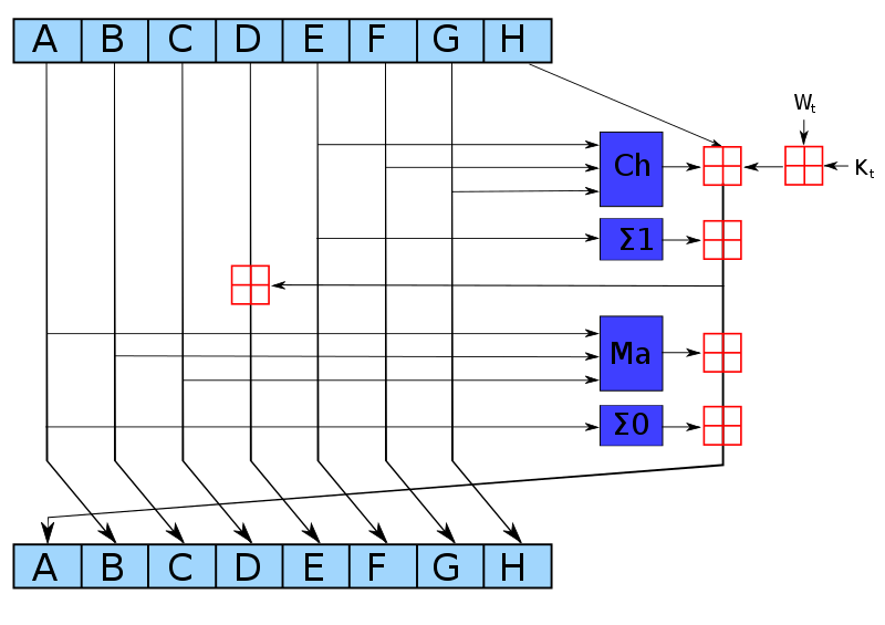
Define as a table mapping a -bit input to an output interleaved with zero bits. We do not require a separate table for range checks because can be used.
Modular addition
To implement addition modulo , we note that this is equivalent to adding the operands using field addition, and then masking away all but the lowest 32 bits of the result. For example, if we have two operands and :
we decompose each operand (along with the result) into 16-bit chunks:
and then reformulate the constraint using field addition:
More generally, any bit-decomposition of the output can be used, not just a decomposition into 16-bit chunks. Note that this correctly handles the carry from .
This constraint requires that each chunk is correctly range-checked (or else an assignment could overflow the field).
-
The operand and result chunks can be constrained using , by looking up each chunk in the "dense" column within a subset of the table. This way we additionally get the "spread" form of the output for free; in particular this is true for the output of the bottom-right which becomes , and the output of the leftmost which becomes . We will use this below to optimize and .
-
must be constrained to the precise range of allowed carry values for the number of operands. We do this with a small range constraint.
Maj function
can be done in lookups: chunks
- As mentioned above, after the first round we already have in spread form . Similarly, and are equal to the and respectively of the previous round, and therefore in the steady state we already have them in spread form and . In fact we can also assume we have them in spread form in the first round, either from the fixed IV or from the use of to reduce the output of the feedforward in the previous block.
- Add the spread forms in the field: ;
- We can add them as -bit words or in pieces; it's equivalent
- Witness the compressed even bits and the compressed odd bits for ;
- Constrain , where is the function output.
Note: by "even" bits we mean the bits of weight an even-power of , i.e. of weight . Similarly by "odd" bits we mean the bits of weight an odd-power of .
Ch function
TODO: can probably be optimised to or lookups using an additional table.
can be done in lookups: chunks
- As mentioned above, after the first round we already have in spread form . Similarly, and are equal to the and respectively of the previous round, and therefore in the steady state we already have them in spread form and . In fact we can also assume we have them in spread form in the first round, either from the fixed IV or from the use of to reduce the output of the feedforward in the previous block.
- Calculate and , where .
- We can add them as -bit words or in pieces; it's equivalent.
- works to compute the spread of even though negation and do not commute in general. It works because each spread bit in is subtracted from , so there are no borrows.
- Witness such that , and similarly for .
- is the function output.
Σ_0 function
can be done in lookups.
To achieve this we first split into pieces , of lengths bits respectively counting from the little end. At the same time we obtain the spread forms of these pieces. This can all be done in two PLONK rows, because the and -bit pieces can be handled using lookups, and the -bit piece can be split into -bit subpieces. The latter and the remaining -bit piece can be range-checked by polynomial constraints in parallel with the two lookups, two small pieces in each row. The spread forms of these small pieces are found by interpolation.
Note that the splitting into pieces can be combined with the reduction of , i.e. no extra lookups are needed for the latter. In the last round we reduce after adding the feedforward (requiring a carry of up to which is fine).
is equivalent to :
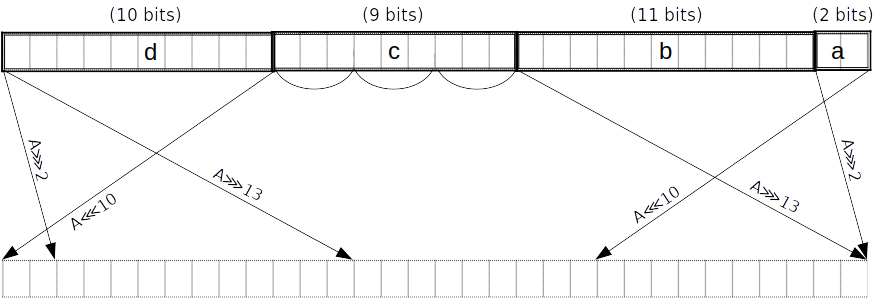
Then, using more lookups we obtain the result as the even bits of a linear combination of the pieces:
That is, we witness the compressed even bits and the compressed odd bits , and constrain where is the function output.
Σ_1 function
can be done in lookups.
To achieve this we first split into pieces , of lengths bits respectively counting from the little end. At the same time we obtain the spread forms of these pieces. This can all be done in two PLONK rows, because the and -bit pieces can be handled using lookups, the -bit piece can be split into and -bit subpieces, and the -bit piece can be split into -bit subpieces. The four small pieces can be range-checked by polynomial constraints in parallel with the two lookups, two small pieces in each row. The spread forms of these small pieces are found by interpolation.
Note that the splitting into pieces can be combined with the reduction of , i.e. no extra lookups are needed for the latter. In the last round we reduce after adding the feedforward (requiring a carry of up to which is fine).
is equivalent to .
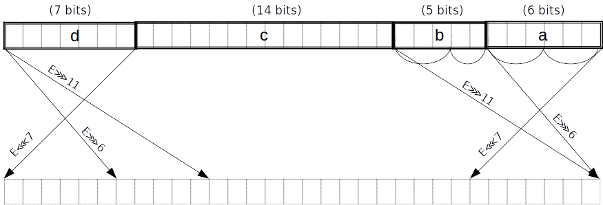
Then, using more lookups we obtain the result as the even bits of a linear combination of the pieces, in the same way we did for :
That is, we witness the compressed even bits and the compressed odd bits , and constrain where is the function output.
Block decomposition
For each block of the padded message, words of bits each are constructed as follows:
- The first are obtained by splitting into -bit blocks
- The remaining words are constructed using the formula: for .
Note: -based numbering is used for the word indices.
Note: is a right-shift, not a rotation.
σ_0 function
is equivalent to .
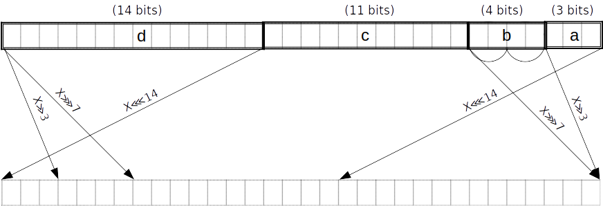
As above but with pieces of lengths counting from the little end. Split into two -bit subpieces.
σ_1 function
is equivalent to .
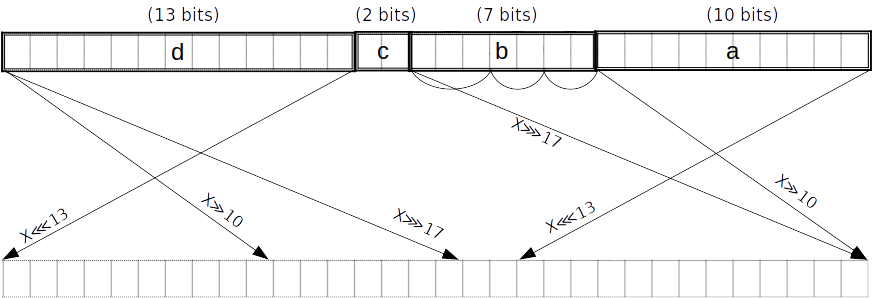
TODO: this diagram doesn't match the expression on the right. This is just for consistency with the other diagrams.
As above but with pieces of lengths counting from the little end. Split into -bit subpieces.
Message scheduling
We apply to , and to . In order to avoid redundant applications of , we can merge the splitting into pieces for and in the case of . Merging the piece lengths and gives pieces of lengths .
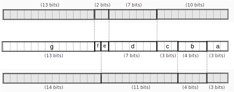
If we can do the merged split in rows (as opposed to a total of rows when splitting for and separately), we save rows.
These might even be doable in rows; not sure. —Daira
We can merge the reduction mod of into their splitting when they are used to compute subsequent words, similarly to what we did for and in the round function.
We will still need to reduce since they are not split. (Technically we could leave them unreduced since they will be reduced later when they are used to compute and -- but that would require handling a carry of up to rather than , so it's not worth the complexity.)
The resulting message schedule cost is:
- rows to constrain to bits
- This is technically optional, but let's do it for robustness, since the rest of the input is constrained for free.
- rows to split into -bit pieces
- rows to split into -bit pieces (merged with a reduction for )
- rows to split into -bit pieces (merged with a reduction)
- rows to extract the results of for
- rows to extract the results of for
- rows to reduce
- rows.
Overall cost
For each round:
- rows for
- rows for
- rows for
- rows for
- and are always free
- per round
This gives rows for all of "step 3", to which we need to add:
- rows for message scheduling
- rows for reductions mod in "step 4"
giving a total of rows.
Tables
We only require one table , with rows and columns. We need a tag column to allow selecting -bit subsets of the table for and .
spread table
| row | tag | table (16b) | spread (32b) |
|---|---|---|---|
| 0 | 0000000000000000 | 00000000000000000000000000000000 | |
| 0 | 0000000000000001 | 00000000000000000000000000000001 | |
| 0 | 0000000000000010 | 00000000000000000000000000000100 | |
| 0 | 0000000000000011 | 00000000000000000000000000000101 | |
| ... | 0 | ... | ... |
| 0 | 0000000001111111 | 00000000000000000001010101010101 | |
| 1 | 0000000010000000 | 00000000000000000100000000000000 | |
| ... | 1 | ... | ... |
| 1 | 0000001111111111 | 00000000000001010101010101010101 | |
| ... | 2 | ... | ... |
| 2 | 0000011111111111 | 00000000010101010101010101010101 | |
| ... | 3 | ... | ... |
| 3 | 0001111111111111 | 00000001010101010101010101010101 | |
| ... | 4 | ... | ... |
| 4 | 0011111111111111 | 00000101010101010101010101010101 | |
| ... | 5 | ... | ... |
| 5 | 1111111111111111 | 01010101010101010101010101010101 |
For example, to do an -bit lookup, we polynomial-constrain the tag to be in . For the most common case of a -bit lookup, we don't need to constrain the tag. Note that we can fill any unused rows beyond with a duplicate entry, e.g. all-zeroes.
Gates
Choice gate
Input from previous operations:
- 64-bit spread forms of 32-bit words , assumed to be constrained by previous operations
- in practice, we'll have the spread forms of after they've been decomposed into 16-bit subpieces
- is defined as
E ∧ F
| s_ch | |||||
|---|---|---|---|---|---|
| 0 | {0,1,2,3,4,5} | ||||
| 1 | {0,1,2,3,4,5} | ||||
| 0 | {0,1,2,3,4,5} | ||||
| 0 | {0,1,2,3,4,5} |
¬E ∧ G
| s_ch_neg | ||||||
|---|---|---|---|---|---|---|
| 0 | {0,1,2,3,4,5} | |||||
| 1 | {0,1,2,3,4,5} | |||||
| 0 | {0,1,2,3,4,5} | |||||
| 0 | {0,1,2,3,4,5} |
Constraints:
s_ch(choice):s_ch_neg(negation):s_chwith an extra negation check- lookup on
- permutation between
Output:
Majority gate
Input from previous operations:
- 64-bit spread forms of 32-bit words , assumed to be constrained by previous operations
- in practice, we'll have the spread forms of after they've been decomposed into -bit subpieces
| s_maj | ||||||
|---|---|---|---|---|---|---|
| 0 | {0,1,2,3,4,5} | |||||
| 1 | {0,1,2,3,4,5} | |||||
| 0 | {0,1,2,3,4,5} | |||||
| 0 | {0,1,2,3,4,5} |
Constraints:
s_maj(majority):- lookup on
- permutation between
Output:
Σ_0 gate
is a 32-bit word split into -bit chunks, starting from the little end. We refer to these chunks as respectively, and further split into three 3-bit chunks . We witness the spread versions of the small chunks.
| s_upp_sigma_0 | |||||||
|---|---|---|---|---|---|---|---|
| 0 | {0,1,2,3,4,5} | ||||||
| 1 | {0,1,2,3,4,5} | ||||||
| 0 | {0,1,2,3,4,5} | ||||||
| 0 | {0,1,2,3,4,5} |
Constraints:
s_upp_sigma_0( constraint):
- lookup on
- 2-bit range check and 2-bit spread check on
- 3-bit range check and 3-bit spread check on
(see section Helper gates)
Output:
Σ_1 gate
is a 32-bit word split into -bit chunks, starting from the little end. We refer to these chunks as respectively, and further split into two 3-bit chunks and into (2,3)-bit chunks . We witness the spread versions of the small chunks.
| s_upp_sigma_1 | ||||||||
|---|---|---|---|---|---|---|---|---|
| 0 | {0,1,2,3,4,5} | |||||||
| 1 | {0,1,2,3,4,5} | |||||||
| 0 | {0,1,2,3,4,5} | |||||||
| 0 | {0,1,2,3,4,5} |
Constraints:
s_upp_sigma_1( constraint):
- lookup on
- 2-bit range check and 2-bit spread check on
- 3-bit range check and 3-bit spread check on
(see section Helper gates)
Output:
σ_0 gate
v1
v1 of the gate takes in a word that's split into -bit chunks (already constrained by message scheduling). We refer to these chunks respectively as is further split into two 2-bit chunks We witness the spread versions of the small chunks. We already have and from the message scheduling.
is equivalent to .
| s_low_sigma_0 | |||||||
|---|---|---|---|---|---|---|---|
| 0 | {0,1,2,3,4,5} | ||||||
| 1 | {0,1,2,3,4,5} | ||||||
| 0 | {0,1,2,3,4,5} | ||||||
| 0 | {0,1,2,3,4,5} |
Constraints:
s_low_sigma_0( v1 constraint):
- check that
bwas properly split into subsections for 4-bit pieces. - 2-bit range check and 2-bit spread check on
- 3-bit range check and 3-bit spread check on
v2
v2 of the gate takes in a word that's split into -bit chunks (already constrained by message scheduling). We refer to these chunks respectively as We already have from the message scheduling. The 1-bit remain unchanged by the spread operation and can be used directly. We further split into two 2-bit chunks We witness the spread versions of the small chunks.
is equivalent to .
| s_low_sigma_0_v2 | ||||||||
|---|---|---|---|---|---|---|---|---|
| 0 | {0,1,2,3,4,5} | |||||||
| 1 | {0,1,2,3,4,5} | |||||||
| 0 | {0,1,2,3,4,5} | |||||||
| 0 | {0,1,2,3,4,5} |
Constraints:
s_low_sigma_0_v2( v2 constraint):
- check that
bwas properly split into subsections for 4-bit pieces. - 2-bit range check and 2-bit spread check on
- 3-bit range check and 3-bit spread check on
σ_1 gate
v1
v1 of the gate takes in a word that's split into -bit chunks (already constrained by message scheduling). We refer to these chunks respectively as is further split into -bit chunks We witness the spread versions of the small chunks. We already have and from the message scheduling.
is equivalent to .
| s_low_sigma_1 | |||||||
|---|---|---|---|---|---|---|---|
| 0 | {0,1,2,3,4,5} | ||||||
| 1 | {0,1,2,3,4,5} | ||||||
| 0 | {0,1,2,3,4,5} | ||||||
| 0 | {0,1,2,3,4,5} |
Constraints:
-
s_low_sigma_1( v1 constraint): -
check that
bwas properly split into subsections for 7-bit pieces. -
2-bit range check and 2-bit spread check on
-
3-bit range check and 3-bit spread check on
v2
v2 of the gate takes in a word that's split into -bit chunks (already constrained by message scheduling). We refer to these chunks respectively as We already have from the message scheduling. The 1-bit remain unchanged by the spread operation and can be used directly. We further split into two 2-bit chunks We witness the spread versions of the small chunks.
is equivalent to .
| s_low_sigma_1_v2 | ||||||||
|---|---|---|---|---|---|---|---|---|
| 0 | {0,1,2,3,4,5} | |||||||
| 1 | {0,1,2,3,4,5} | |||||||
| 0 | {0,1,2,3,4,5} | |||||||
| 0 | {0,1,2,3,4,5} |
Constraints:
s_low_sigma_1_v2( v2 constraint):
- check that
bwas properly split into subsections for 4-bit pieces. - 2-bit range check and 2-bit spread check on
- 3-bit range check and 3-bit spread check on
Helper gates
Small range constraints
Let . Constraining this expression to equal zero enforces that is in
2-bit range check
| sr2 | |
|---|---|
| 1 | a |
2-bit spread
| ss2 | ||
|---|---|---|
| 1 | a | a' |
with interpolation polynomials:
- ()
- ()
- ()
- ()
3-bit range check
| sr3 | |
|---|---|
| 1 | a |
3-bit spread
| ss3 | ||
|---|---|---|
| 1 | a | a' |
with interpolation polynomials:
- ()
- ()
- ()
- ()
- ()
- ()
- ()
- ()
reduce_6 gate
Addition of 6 elements
Input:
Check:
Assume inputs are constrained to 16 bits.
- Addition gate (sa):
- Carry gate (sc):
| sa | sc | ||||||||
|---|---|---|---|---|---|---|---|---|---|
| 1 | 0 | ||||||||
| 1 | 1 |
Assume inputs are constrained to 16 bits.
- Addition gate (sa):
- Carry gate (sc):
| sa | sc | ||||
|---|---|---|---|---|---|
| 0 | 0 | ||||
| 1 | 1 | ||||
| 0 | 0 | ||||
| 1 | 0 |
reduce_7 gate
Addition of 7 elements
Input:
Check:
Assume inputs are constrained to 16 bits.
- Addition gate (sa):
- Carry gate (sc):
| sa | sc | |||||||||
|---|---|---|---|---|---|---|---|---|---|---|
| 1 | 0 | |||||||||
| 1 | 1 |
Message scheduling region
For each block of the padded message, words of bits each are constructed as follows:
- the first are obtained by splitting into -bit blocks
- the remaining words are constructed using the formula: for .
| sw | sd0 | sd1 | sd2 | sd3 | ss0 | ss0_v2 | ss1 | ss1_v2 | ||||||||||
|---|---|---|---|---|---|---|---|---|---|---|---|---|---|---|---|---|---|---|
| 0 | 1 | 0 | 0 | 0 | 0 | 0 | 0 | 0 | {0,1,2,3,4,5} | |||||||||
| 1 | 0 | 0 | 0 | 0 | 0 | 0 | 0 | 0 | {0,1,2,3,4,5} | |||||||||
| 0 | 1 | 1 | 0 | 0 | 0 | 0 | 0 | 0 | {0,1,2,3,4} | |||||||||
| 1 | 0 | 0 | 0 | 0 | 0 | 0 | 0 | 0 | {0,1,2} | |||||||||
| 0 | 0 | 0 | 0 | 0 | 0 | 0 | 0 | 0 | {0,1,2,3,4,5} | |||||||||
| 0 | 0 | 0 | 0 | 0 | 1 | 0 | 0 | 0 | {0,1,2,3,4,5} | |||||||||
| 0 | 0 | 0 | 0 | 0 | 0 | 0 | 0 | 0 | {0,1,2,3,4,5} | |||||||||
| 0 | 0 | 0 | 0 | 0 | 0 | 0 | 0 | 0 | {0,1,2,3,4,5} | |||||||||
| .. | ... | ... | ... | ... | ... | ... | ... | ... | ... | ... | ... | ... | ... | ... | ... | ... | ... | |
| 0 | 0 | 0 | 0 | 0 | 0 | 0 | 0 | 0 | {0,1,2,3} | |||||||||
| 0 | 1 | 0 | 1 | 0 | 0 | 0 | 0 | 0 | 0 | |||||||||
| 1 | 0 | 0 | 0 | 0 | 0 | 0 | 0 | 0 | 0 | |||||||||
| 0 | 0 | 0 | 0 | 0 | 0 | 0 | 0 | 0 | {0,1,2,3,4,5} | |||||||||
| 0 | 0 | 0 | 0 | 0 | 0 | 1 | 0 | 0 | {0,1,2,3,4,5} | |||||||||
| 0 | 0 | 0 | 0 | 0 | 0 | 0 | 0 | 0 | {0,1,2,3,4,5} | |||||||||
| 0 | 0 | 0 | 0 | 0 | 0 | 0 | 0 | 0 | {0,1,2,3,4,5} | |||||||||
| 0 | 0 | 0 | 0 | 0 | 0 | 0 | 0 | 0 | {0,1,2,3,4,5} | |||||||||
| 0 | 0 | 0 | 0 | 0 | 0 | 0 | 0 | 1 | {0,1,2,3,4,5} | |||||||||
| 0 | 0 | 0 | 0 | 0 | 0 | 0 | 0 | 0 | {0,1,2,3,4,5} | |||||||||
| 0 | 0 | 0 | 0 | 0 | 0 | 0 | 0 | 0 | {0,1,2,3,4,5} | |||||||||
| .. | ... | ... | ... | ... | ... | ... | ... | ... | ... | ... | ... | ... | ... | ... | ... | ... | ... | |
| 0 | 1 | 0 | 0 | 1 | 0 | 0 | 0 | 0 | {0,1,2,3} | |||||||||
| 0 | 0 | 0 | 0 | 0 | 0 | 0 | 0 | 0 | {0,1} | |||||||||
| 0 | 0 | 0 | 0 | 0 | 0 | 0 | 0 | 0 | {0,1,2,3,4,5} | |||||||||
| 0 | 0 | 0 | 0 | 0 | 0 | 0 | 0 | 1 | {0,1,2,3,4,5} | |||||||||
| 0 | 0 | 0 | 0 | 0 | 0 | 0 | 0 | 0 | {0,1,2,3,4,5} | |||||||||
| 0 | 0 | 0 | 0 | 0 | 0 | 0 | 0 | 0 | {0,1,2,3,4,5} | |||||||||
| .. | ... | ... | ... | ... | ... | ... | ... | ... | ... | ... | ... | ... | ... | ... | ... | ... | ... | |
| 0 | 1 | 0 | 0 | 0 | 0 | 0 | 0 | 0 | {0,1,2,3,4,5} | |||||||||
| 0 | 0 | 0 | 0 | 0 | 0 | 0 | 0 | 0 | {0,1,2,3,4,5} | |||||||||
| 0 | 1 | 0 | 0 | 0 | 0 | 0 | 0 | 0 | {0,1,2,3,4,5} | |||||||||
| 0 | 0 | 0 | 0 | 0 | 0 | 0 | 0 | 0 | {0,1,2,3,4,5} |
Constraints:
sw: construct word usingsd0: decomposition gate forsd1: decomposition gate for (split into -bit pieces)sd2: decomposition gate for (split into -bit pieces)sd3: decomposition gate for (split into -bit pieces)
Compression region
+----------------------------------------------------------+
|                                                          |
|          decompose E,                                    |
|          Σ_1(E)                                          |
|                                                          |
|                  +---------------------------------------+
|                  |                                       |
|                  |        reduce_5() to get H'           |
|                  |                                       |
+----------------------------------------------------------+
|          decompose F, decompose G                        |
|                                                          |
|                        Ch(E,F,G)                         |
|                                                          |
+----------------------------------------------------------+
|                                                          |
|          decompose A,                                    |
|          Σ_0(A)                                          |
|                                                          |
|                                                          |
|                  +---------------------------------------+
|                  |                                       |
|                  |        reduce_7() to get A_new,       |
|                  |              using H'                 |
|                  |                                       |
+------------------+---------------------------------------+
|          decompose B, decompose C                        |
|                                                          |
|          Maj(A,B,C)                                      |
|                                                          |
|                  +---------------------------------------+
|                  |        reduce_6() to get E_new,       |
|                  |              using H'                 |
+------------------+---------------------------------------+
Initial round:
| s_digest | sd_abcd | sd_efgh | ss0 | ss1 | s_maj | s_ch_neg | s_ch | s_a_new | s_e_new | s_h_prime | ||||||||||
|---|---|---|---|---|---|---|---|---|---|---|---|---|---|---|---|---|---|---|---|---|
| 0 | 0 | 1 | 0 | 0 | 0 | 0 | 0 | 0 | 0 | 0 | {0,1,2} | |||||||||
| 0 | 0 | 0 | 0 | 0 | 0 | 0 | 0 | 0 | 0 | 0 | {0,1} | |||||||||
| 0 | 0 | 0 | 0 | 0 | 0 | 0 | 0 | 0 | 0 | 0 | {0,1,2,3,4,5} | |||||||||
| 0 | 0 | 0 | 0 | 1 | 0 | 0 | 0 | 0 | 0 | 0 | {0,1,2,3,4,5} | |||||||||
| 0 | 0 | 0 | 0 | 0 | 0 | 0 | 0 | 0 | 0 | 0 | {0,1,2,3,4,5} | |||||||||
| 0 | 0 | 0 | 0 | 0 | 0 | 0 | 0 | 0 | 0 | 0 | {0,1,2,3,4,5} | |||||||||
| 0 | 0 | 1 | 0 | 0 | 0 | 0 | 0 | 0 | 0 | 0 | {0,1,2} | |||||||||
| 0 | 0 | 0 | 0 | 0 | 0 | 0 | 0 | 0 | 0 | 0 | {0,1} | |||||||||
| 0 | 0 | 1 | 0 | 0 | 0 | 0 | 0 | 0 | 0 | 0 | {0,1,2} | |||||||||
| 0 | 0 | 0 | 0 | 0 | 0 | 0 | 0 | 0 | 0 | 0 | {0,1} | |||||||||
| 0 | 0 | 0 | 0 | 0 | 0 | 0 | 0 | 0 | 0 | 0 | {0,1,2,3,4,5} | |||||||||
| 0 | 0 | 0 | 0 | 0 | 0 | 0 | 1 | 0 | 0 | 1 | {0,1,2,3,4,5} | |||||||||
| 0 | 0 | 0 | 0 | 0 | 0 | 0 | 0 | 0 | 0 | 0 | {0,1,2,3,4,5} | |||||||||
| 0 | 0 | 0 | 0 | 0 | 0 | 0 | 0 | 0 | 0 | 0 | {0,1,2,3,4,5} | |||||||||
| 0 | 0 | 0 | 0 | 0 | 0 | 0 | 0 | 0 | 1 | 0 | {0,1,2,3,4,5} | |||||||||
| 0 | 0 | 0 | 0 | 0 | 0 | 1 | 0 | 0 | 0 | 0 | {0,1,2,3,4,5} | |||||||||
| 0 | 0 | 0 | 0 | 0 | 0 | 0 | 0 | 0 | 0 | 0 | {0,1,2,3,4,5} | |||||||||
| 0 | 0 | 0 | 0 | 0 | 0 | 0 | 0 | 0 | 0 | 0 | {0,1,2,3,4,5} | |||||||||
| 0 | 1 | 0 | 0 | 0 | 0 | 0 | 0 | 0 | 0 | 0 | {0,1,2} | |||||||||
| 0 | 0 | 0 | 0 | 0 | 0 | 0 | 0 | 0 | 0 | 0 | {0,1} | |||||||||
| 0 | 0 | 0 | 0 | 0 | 0 | 0 | 0 | 0 | 0 | 0 | {0,1,2,3,4,5} | |||||||||
| 0 | 0 | 0 | 1 | 0 | 0 | 0 | 0 | 0 | 0 | 0 | {0,1,2,3,4,5} | |||||||||
| 0 | 0 | 0 | 0 | 0 | 0 | 0 | 0 | 0 | 0 | 0 | {0,1,2,3,4,5} | |||||||||
| 0 | 0 | 0 | 0 | 0 | 0 | 0 | 0 | 0 | 0 | 0 | {0,1,2,3,4,5} | |||||||||
| 0 | 1 | 0 | 0 | 0 | 0 | 0 | 0 | 0 | 0 | 0 | {0,1,2} | |||||||||
| 0 | 0 | 0 | 0 | 0 | 0 | 0 | 0 | 0 | 0 | 0 | {0,1} | |||||||||
| 0 | 1 | 0 | 0 | 0 | 0 | 0 | 0 | 0 | 0 | 0 | {0,1,2} | |||||||||
| 0 | 0 | 0 | 0 | 0 | 0 | 0 | 0 | 0 | 0 | 0 | {0,1} | |||||||||
| 0 | 0 | 0 | 0 | 0 | 0 | 0 | 0 | 0 | 0 | 0 | {0,1,2,3,4,5} | |||||||||
| 0 | 0 | 0 | 0 | 0 | 1 | 0 | 0 | 1 | 0 | 0 | {0,1,2,3,4,5} | |||||||||
| 0 | 0 | 0 | 0 | 0 | 0 | 0 | 0 | 0 | 0 | 0 | {0,1,2,3,4,5} | |||||||||
| 0 | 0 | 0 | 0 | 0 | 0 | 0 | 0 | 0 | 0 | 0 | {0,1,2,3,4,5} |
Steady-state:
| s_digest | sd_abcd | sd_efgh | ss0 | ss1 | s_maj | s_ch_neg | s_ch | s_a_new | s_e_new | s_h_prime | ||||||||||
|---|---|---|---|---|---|---|---|---|---|---|---|---|---|---|---|---|---|---|---|---|
| 0 | 0 | 1 | 0 | 0 | 0 | 0 | 0 | 0 | 0 | 0 | {0,1,2} | |||||||||
| 0 | 0 | 0 | 0 | 0 | 0 | 0 | 0 | 0 | 0 | 0 | {0,1} | |||||||||
| 0 | 0 | 0 | 0 | 0 | 0 | 0 | 0 | 0 | 0 | 0 | {0,1,2,3,4,5} | |||||||||
| 0 | 0 | 0 | 0 | 1 | 0 | 0 | 0 | 0 | 0 | 0 | {0,1,2,3,4,5} | |||||||||
| 0 | 0 | 0 | 0 | 0 | 0 | 0 | 0 | 0 | 0 | 0 | {0,1,2,3,4,5} | |||||||||
| 0 | 0 | 0 | 0 | 0 | 0 | 0 | 0 | 0 | 0 | 0 | {0,1,2,3,4,5} | |||||||||
| 0 | 0 | 0 | 0 | 0 | 0 | 0 | 0 | 0 | 0 | 0 | {0,1,2,3,4,5} | |||||||||
| 0 | 0 | 0 | 0 | 0 | 0 | 0 | 1 | 0 | 0 | 1 | {0,1,2,3,4,5} | |||||||||
| 0 | 0 | 0 | 0 | 0 | 0 | 0 | 0 | 0 | 0 | 0 | {0,1,2,3,4,5} | |||||||||
| 0 | 0 | 0 | 0 | 0 | 0 | 0 | 0 | 0 | 0 | 0 | {0,1,2,3,4,5} | |||||||||
| 0 | 0 | 0 | 0 | 0 | 0 | 0 | 0 | 0 | 1 | 0 | {0,1,2,3,4,5} | |||||||||
| 0 | 0 | 0 | 0 | 0 | 0 | 1 | 0 | 0 | 0 | 0 | {0,1,2,3,4,5} | |||||||||
| 0 | 0 | 0 | 0 | 0 | 0 | 0 | 0 | 0 | 0 | 0 | {0,1,2,3,4,5} | |||||||||
| 0 | 0 | 0 | 0 | 0 | 0 | 0 | 0 | 0 | 0 | 0 | {0,1,2,3,4,5} | |||||||||
| 0 | 1 | 0 | 0 | 0 | 0 | 0 | 0 | 0 | 0 | 0 | {0,1,2} | |||||||||
| 0 | 0 | 0 | 0 | 0 | 0 | 0 | 0 | 0 | 0 | 0 | {0,1} | |||||||||
| 0 | 0 | 0 | 0 | 0 | 0 | 0 | 0 | 0 | 0 | 0 | {0,1,2,3,4,5} | |||||||||
| 0 | 0 | 0 | 1 | 0 | 0 | 0 | 0 | 0 | 0 | 0 | {0,1,2,3,4,5} | |||||||||
| 0 | 0 | 0 | 0 | 0 | 0 | 0 | 0 | 0 | 0 | 0 | {0,1,2,3,4,5} | |||||||||
| 0 | 0 | 0 | 0 | 0 | 0 | 0 | 0 | 0 | 0 | 0 | {0,1,2,3,4,5} | |||||||||
| 0 | 0 | 0 | 0 | 0 | 0 | 0 | 0 | 0 | 0 | 0 | {0,1,2,3,4,5} | |||||||||
| 0 | 0 | 0 | 0 | 0 | 1 | 0 | 0 | 1 | 0 | 0 | {0,1,2,3,4,5} | |||||||||
| 0 | 0 | 0 | 0 | 0 | 0 | 0 | 0 | 0 | 0 | 0 | {0,1,2,3,4,5} | |||||||||
| 0 | 0 | 0 | 0 | 0 | 0 | 0 | 0 | 0 | 0 | 0 | {0,1,2,3,4,5} |
Final digest:
| s_digest | sd_abcd | sd_efgh | ss0 | ss1 | s_maj | s_ch_neg | s_ch | s_a_new | s_e_new | s_h_prime | ||||||||||
|---|---|---|---|---|---|---|---|---|---|---|---|---|---|---|---|---|---|---|---|---|
| 1 | 0 | 0 | 0 | 0 | 0 | 0 | 0 | 0 | 0 | 0 | 0 | 0 | 0 | |||||||
| 0 | 0 | 0 | 0 | 0 | 0 | 0 | 0 | 0 | 0 | 0 | 0 | 0 | 0 | |||||||
| 1 | 0 | 0 | 0 | 0 | 0 | 0 | 0 | 0 | 0 | 0 | 0 | 0 | 0 | |||||||
| 0 | 0 | 0 | 0 | 0 | 0 | 0 | 0 | 0 | 0 | 0 | 0 | 0 | 0 |
Background Material
This section covers the background material required to understand the Halo 2 proving system. It is targeted at an ELI15 (Explain It Like I'm 15) level; if you think anything could do with additional explanation, let us know!
Fields
A fundamental component of many cryptographic protocols is the algebraic structure known as a field. Fields are sets of objects (usually numbers) with two associated binary operators and such that various field axioms hold. The real numbers are an example of a field with an uncountably infinite number of elements.
Halo makes use of finite fields which have a finite number of elements. Finite fields are fully classified as follows:
- if is a finite field, it contains elements for some integer and some prime ;
- any two finite fields with the same number of elements are isomorphic. In particular, all of the arithmetic in a prime field is isomorphic to addition and multiplication of integers modulo , i.e. in . This is why we often refer to as the modulus.
We'll write a field as where . The prime is called its characteristic. In the cases where the field is a -degree extension of the field . (By analogy, the complex numbers are an extension of the real numbers.) However, in Halo we do not use extension fields. Whenever we write we are referring to what we call a prime field which has a prime number of elements, i.e. .
Important notes:
- There are two special elements in any field: , the additive identity, and , the multiplicative identity.
- The least significant bit of a field element, when represented as an integer in binary format, can be interpreted as its "sign" to help distinguish it from its additive inverse (negation). This is because for some nonzero element which has a least significant bit we have that has a least significant bit , and vice versa. We could also use whether or not an element is larger than to give it a "sign."
Finite fields will be useful later for constructing polynomials and elliptic curves. Elliptic curves are examples of groups, which we discuss next.
Groups
Groups are simpler and more limited than fields; they have only one binary operator and fewer axioms. They also have an identity, which we'll denote as .
Any non-zero element in a group has an inverse , which is the unique element such that .
For example, the set of nonzero elements of forms a group, where the group operation is given by multiplication on the field.
(aside) Additive vs multiplicative notation
If is written as or omitted (i.e. written as ), the identity as , and inversion as , as we did above, then we say that the group is "written multiplicatively". If is written as , the identity as or , and inversion as , then we say it is "written additively".
It's conventional to use additive notation for elliptic curve groups, and multiplicative notation when the elements come from a finite field.
When additive notation is used, we also write
for nonnegative and call this "scalar multiplication"; we also often use uppercase letters for variables denoting group elements. When multiplicative notation is used, we also write
and call this "exponentiation". In either case we call the scalar such that or the "discrete logarithm" of to base . We can extend scalars to negative integers by inversion, i.e. or .
The order of an element of a finite group is defined as the smallest positive integer such that (in multiplicative notation) or (in additive notation). The order of the group is the number of elements.
Groups always have a generating set, which is a set of elements such that we can produce any element of the group as (in multiplicative terminology) a product of powers of those elements. So if the generating set is , we can produce any element of the group as . There can be many different generating sets for a given group.
A group is called cyclic if it has a (not necessarily unique) generating set with only a single element — call it . In that case we can say that generates the group, and that the order of is the order of the group.
Any finite cyclic group of order is isomorphic to the integers modulo (denoted ), such that:
- the operation in corresponds to addition modulo ;
- the identity in corresponds to ;
- some generator corresponds to .
Given a generator , the isomorphism is always easy to compute in the direction; it is just (or in additive notation, ). It may be difficult in general to compute in the direction; we'll discuss this further when we come to elliptic curves.
If the order of a finite group is prime, then the group is cyclic, and every non-identity element is a generator.
The multiplicative group of a finite field
We use the notation for the multiplicative group (i.e. the group operation is multiplication in ) over the set .
A quick way of obtaining the inverse in is . The reason for this stems from Fermat's little theorem, which states that for any integer . If is nonzero, we can divide by twice to get
Let's assume that is a generator of , so it has order (equal to the number of elements in ). Therefore, for any element in there is a unique integer such that .
Notice that where can really be interpreted as where and . Indeed, it holds that for all . As a result the multiplication of nonzero field elements can be interpreted as addition modulo with respect to some fixed generator . The addition just happens "in the exponent."
This is another way to look at where comes from for computing inverses in the field:
so .
Montgomery's Trick
Montgomery's trick, named after Peter Montgomery (RIP) is a way to compute many group inversions at the same time. It is commonly used to compute inversions in , which are quite computationally expensive compared to multiplication.
Imagine we need to compute the inverses of three nonzero elements . Instead, we'll compute the products and , and compute the inversion
We can now multiply by to obtain and multiply by to obtain , which we can then multiply by to obtain their respective inverses.
This technique generalizes to arbitrary numbers of group elements with just a single inversion necessary.
Multiplicative subgroups
A subgroup of a group with operation , is a subset of elements of that also form a group under .
In the previous section we said that is a generator of the -order multiplicative group . This group has composite order, and so by the Chinese remainder theorem1 it has strict subgroups. As an example let's imagine that , and so factors into . Thus, there is a generator of the -order subgroup and a generator of the -order subgroup. All elements in , therefore, can be written uniquely as for some (modulo ) and some (modulo ).
If we have notice what happens when we compute
we have effectively "killed" the -order subgroup component, producing a value in the -order subgroup.
Lagrange's theorem (group theory) states that the order of any subgroup of a finite group divides the order of . Therefore, the order of any subgroup of must divide
Square roots
In a field exactly half of all nonzero elements are squares; the remainder are non-squares or "quadratic non-residues". In order to see why, consider an that generates the -order multiplicative subgroup of (this exists because is divisible by since is a prime greater than ) and that generates the -order multiplicative subgroup of where . Then every element can be written uniquely as with and . Half of all elements will have and the other half will have .
Let's consider the simple case where and so is odd (if is even, then would be divisible by , which contradicts being ). If is a square, then there must exist such that . But this means that
In other words, all squares in this particular field do not generate the -order multiplicative subgroup, and so since half of the elements generate the -order subgroup then at most half of the elements are square. In fact exactly half of the elements are square (since squaring each nonsquare element gives a unique square). This means we can assume all squares can be written as for some , and therefore finding the square root is a matter of exponentiating by .
In the event that then things get more complicated because does not exist. Let's write as with odd. The case is impossible, and the case is what we already described, so consider . generates a -order multiplicative subgroup and generates the odd -order multiplicative subgroup. Then every element can be written as for and . If the element is a square, then there exists some which can be written for and . This means that , therefore we have , and . would have to be even in this case because otherwise it would be impossible to have for any . In the case that is not a square, then is odd, and so half of all elements are squares.
In order to compute the square root, we can first raise the element to the power to "kill" the -order component, giving
and then raise this result to the power to undo the effect of the original exponentiation on the -order component:
(since is relatively prime to ). This leaves bare the value which we can trivially handle. We can similarly kill the -order component to obtain , and put the values together to obtain the square root.
It turns out that in the cases there are simpler algorithms that merge several of these exponentiations together for efficiency. For other values of , the only known way is to manually extract by squaring until you obtain the identity for every single bit of . This is the essence of the Tonelli-Shanks square root algorithm and describes the general strategy. (There is another square root algorithm that uses quadratic extension fields, but it doesn't pay off in efficiency until the prime becomes quite large.)
Roots of unity
In the previous sections we wrote with odd, and stated that an element generated the -order subgroup. For convenience, let's denote The elements are known as the th roots of unity.
The primitive root of unity, is an th root of unity such that except when .
Important notes:
-
If is an th root of unity, satisfies If then
-
Equivalently, the roots of unity are solutions to the equation
-
("Negation lemma"). Proof: Since the order of is , Therefore,
-
("Halving lemma"). Proof: In other words, if we square each element in the th roots of unity, we would get back only half the elements, (i.e. the th roots of unity). There is a two-to-one mapping between the elements and their squares.
References
Polynomials
Let be a polynomial over with formal indeterminate . As an example,
defines a degree- polynomial. is referred to as the constant term. Polynomials of degree have coefficients. We will often want to compute the result of replacing the formal indeterminate with some concrete value , which we denote by .
In mathematics this is commonly referred to as "evaluating at a point ". The word "point" here stems from the geometrical usage of polynomials in the form , where is the coordinate of a point in two-dimensional space. However, the polynomials we deal with are almost always constrained to equal zero, and will be an element of some field. This should not be confused with points on an elliptic curve, which we also make use of, but never in the context of polynomial evaluation.
Important notes:
- Multiplication of polynomials produces a product polynomial that is the sum of the degrees of its factors. Polynomial division subtracts from the degree.
- Given a polynomial of degree , if we obtain evaluations of the polynomial at distinct points then these evaluations perfectly define the polynomial. In other words, given these evaluations we can obtain a unique polynomial of degree via polynomial interpolation.
- is the coefficient representation of the polynomial . Equivalently, we could use its evaluation representation at distinct points. Either representation uniquely specifies the same polynomial.
(aside) Horner's rule
Horner's rule allows for efficient evaluation of a polynomial of degree , using only multiplications and additions. It is the following identity:
Fast Fourier Transform (FFT)
The FFT is an efficient way of converting between the coefficient and evaluation representations of a polynomial. It evaluates the polynomial at the th roots of unity where is a primitive th root of unity. By exploiting symmetries in the roots of unity, each round of the FFT reduces the evaluation into a problem only half the size. Most commonly we use polynomials of length some power of two, , and apply the halving reduction recursively.
Motivation: Fast polynomial multiplication
In the coefficient representation, it takes operations to multiply two polynomials :
where each of the terms in the first polynomial has to be multiplied by the terms of the second polynomial.
In the evaluation representation, however, polynomial multiplication only requires operations:
where each evaluation is multiplied pointwise.
This suggests the following strategy for fast polynomial multiplication:
- Evaluate polynomials at all points;
- Perform fast pointwise multiplication in the evaluation representation ();
- Convert back to the coefficient representation.
The challenge now is how to evaluate and interpolate the polynomials efficiently. Naively, evaluating a polynomial at points would require operations (we use the Horner's rule at each point):
For convenience, we will denote the matrices above as:
( is known as the Discrete Fourier Transform of ; is also called the Vandermonde matrix.)
The (radix-2) Cooley-Tukey algorithm
Our strategy is to divide a DFT of size into two interleaved DFTs of size . Given the polynomial we split it up into even and odd terms:
To recover the original polynomial, we do
Trying this out on points and , we start to notice some symmetries:
Notice that we are only evaluating and over half the domain (halving lemma). This gives us all the terms we need to reconstruct over the full domain : which means we have transformed a length- DFT into two length- DFTs.
We choose to be a power of two (by zero-padding if needed), and apply this divide-and-conquer strategy recursively. By the Master Theorem1, this gives us an evaluation algorithm with operations, also known as the Fast Fourier Transform (FFT).
Inverse FFT
So we've evaluated our polynomials and multiplied them pointwise. What remains is to convert the product from the evaluation representation back to coefficient representation. To do this, we simply call the FFT on the evaluation representation. However, this time we also:
- replace by in the Vandermonde matrix, and
- multiply our final result by a factor of .
In other words:
(To understand why the inverse FFT has a similar form to the FFT, refer to Slide 13-1 of 2. The below image was also taken from 2.)

The Schwartz-Zippel lemma
The Schwartz-Zippel lemma informally states that "different polynomials are different at most points." Formally, it can be written as follows:
Let be a nonzero polynomial of variables with degree . Let be a finite set of numbers with at least elements in it. If we choose random from ,
In the familiar univariate case , this reduces to saying that a nonzero polynomial of degree has at most roots.
The Schwartz-Zippel lemma is used in polynomial equality testing. Given two multi-variate polynomials and of degrees respectively, we can test if for random where the size of is at least If the two polynomials are identical, this will always be true, whereas if the two polynomials are different then the equality holds with probability at most .
Vanishing polynomial
Consider the order- multiplicative subgroup with primitive root of unity . For all we have In other words, every element of fulfils the equation
meaning every element is a root of We call the vanishing polynomial over because it evaluates to zero on all elements of
This comes in particularly handy when checking polynomial constraints. For instance, to check that over we simply have to check that is some multiple of . In other words, if dividing our constraint by the vanishing polynomial still yields some polynomial we are satisfied that over
Lagrange basis functions
TODO: explain what a basis is in general (briefly).
Polynomials are commonly written in the monomial basis (e.g. ). However, when working over a multiplicative subgroup of order , we find a more natural expression in the Lagrange basis.
Consider the order- multiplicative subgroup with primitive root of unity . The Lagrange basis corresponding to this subgroup is a set of functions , where
We can write this more compactly as where is the Kronecker delta function.
Now, we can write our polynomial as a linear combination of Lagrange basis functions,
which is equivalent to saying that evaluates to at , to at , to at and so on.
When working over a multiplicative subgroup, the Lagrange basis function has a convenient sparse representation of the form
where is the barycentric weight. (To understand how this form was derived, refer to 3.) For we have .
Suppose we are given a set of evaluation points . Since we cannot assume that the 's form a multiplicative subgroup, we consider also the Lagrange polynomials 's in the general case. Then we can construct:
Here, every will produce a zero numerator term causing the whole product to evaluate to zero. On the other hand, will evaluate to at every term, resulting in an overall product of one. This gives the desired Kronecker delta behaviour on the set .
Lagrange interpolation
Given a polynomial in its evaluation representation
we can reconstruct its coefficient form in the Lagrange basis:
where
References
Cryptographic groups
In the section Inverses and groups we introduced the concept of groups. A group has an identity and a group operation. In this section we will write groups additively, i.e. the identity is and the group operation is .
Some groups can be used as cryptographic groups. At the risk of oversimplifying, this means that the problem of finding a discrete logarithm of a group element to a given base , i.e. finding such that , is hard in general.
Pedersen commitment
The Pedersen commitment [P99] is a way to commit to a secret message in a verifiable way. It uses two random public generators where is a cryptographic group of order . A random secret is chosen in , and the message to commit to is from any subset of . The commitment is
To open the commitment, the committer reveals and thus allowing anyone to verify that is indeed a commitment to
Notice that the Pedersen commitment scheme is homomorphic:
Assuming the discrete log assumption holds, Pedersen commitments are also perfectly hiding and computationally binding:
- hiding: the adversary chooses messages The committer commits to one of these messages Given the probability of the adversary guessing the correct is no more than .
- binding: the adversary cannot pick two different messages and randomness such that
Vector Pedersen commitment
We can use a variant of the Pedersen commitment scheme to commit to multiple messages at once, . This time, we'll have to sample a corresponding number of random public generators along with a single random generator as before (for use in hiding). Then, our commitment scheme is:
TODO: is this positionally binding?
Diffie--Hellman
An example of a protocol that uses cryptographic groups is Diffie--Hellman key agreement [DH1976]. The Diffie--Hellman protocol is a method for two users, Alice and Bob, to generate a shared private key. It proceeds as follows:
- Alice and Bob publicly agree on two prime numbers, and where is large and is a primitive root (Note that is a generator of the group )
- Alice chooses a large random number as her private key. She computes her public key and sends to Bob.
- Similarly, Bob chooses a large random number as his private key. He computes his public key and sends to Alice.
- Now both Alice and Bob compute their shared key which Alice computes as and Bob computes as
A potential eavesdropper would need to derive knowing only and : in other words, they would need to either get the discrete logarithm from or from which we assume to be computationally infeasible in
More generally, protocols that use similar ideas to Diffie--Hellman are used throughout cryptography. One way of instantiating a cryptographic group is as an elliptic curve. Before we go into detail on elliptic curves, we'll describe some algorithms that can be used for any group.
Multiscalar multiplication
TODO: Pippenger's algorithm
Reference: https://jbootle.github.io/Misc/pippenger.pdf
Elliptic curves
Elliptic curves constructed over finite fields are another important cryptographic tool.
We use elliptic curves because they provide a cryptographic group, i.e. a group in which the discrete logarithm problem (discussed below) is hard.
There are several ways to define the curve equation, but for our purposes, let be a large (255-bit) field, and then let the set of solutions to for some constant define the -rational points on an elliptic curve . These coordinates are called "affine coordinates". Each of the -rational points, together with a "point at infinity" that serves as the group identity, can be interpreted as an element of a group. By convention, elliptic curve groups are written additively.
 "Three points on a line sum to zero, which is the point at infinity."
The group addition law is simple: to add two points together, find the line that intersects both points and obtain the third point, and then negate its -coordinate. The case that a point is being added to itself, called point doubling, requires special handling: we find the line tangent to the point, and then find the single other point that intersects this line and then negate. Otherwise, in the event that a point is being "added" to its negation, the result is the point at infinity.
The ability to add and double points naturally gives us a way to scale them by integers, called scalars. The number of points on the curve is the group order. If this number is a prime , then the scalars can be considered as elements of a scalar field, .
Elliptic curves, when properly designed, have an important security property. Given two random elements finding such that , otherwise known as the discrete log of with respect to , is considered computationally infeasible with classical computers. This is called the elliptic curve discrete log assumption.
If an elliptic curve group has prime order (like the ones used in Halo 2), then it is a finite cyclic group. Recall from the section on groups that this implies it is isomorphic to , or equivalently, to the scalar field . Each possible generator fixes the isomorphism; then an element on the scalar side is precisely the discrete log of the corresponding group element with respect to . In the case of a cryptographically secure elliptic curve, the isomorphism is hard to compute in the direction because the elliptic curve discrete log problem is hard.
It is sometimes helpful to make use of this isomorphism by thinking of group-based cryptographic protocols and algorithms in terms of the scalars instead of in terms of the group elements. This can make proofs and notation simpler.
For instance, it has become common in papers on proof systems to use the notation to denote a group element with discrete log , where the generator is implicit.
We also used this idea in the "distinct-x theorem", in order to prove correctness of optimizations for elliptic curve scalar multiplication in Sapling, and an endomorphism-based optimization in Appendix C of the original Halo paper.
Curve arithmetic
Point doubling
The simplest situation is doubling a point . Continuing with our example , this is done first by computing the derivative
To obtain expressions for we consider
To get the expression for we substitute into the elliptic curve equation:
Comparing coefficients for the term gives us
Projective coordinates
This unfortunately requires an expensive inversion of . We can avoid this by arranging our equations to "defer" the computation of the inverse, since we often do not need the actual affine coordinate of the resulting point immediately after an individual curve operation. Let's introduce a third coordinate and scale our curve equation by like so:
Our original curve is just this curve at the restriction . If we allow the affine point to be represented by , and then we have the homogenous projective curve
Obtaining from is as simple as computing when . (When we are dealing with the point at infinity .) In this form, we now have a convenient way to defer the inversion required by doubling a point. The general strategy is to express as rational functions using and , rearrange to make their denominators the same, and then take the resulting point to have be the shared denominator and .
Projective coordinates are often, but not always, more efficient than affine coordinates. There may be exceptions to this when either we have a different way to apply Montgomery's trick, or when we're in the circuit setting where multiplications and inversions are about equally as expensive (at least in terms of circuit size).
The following shows an example of doubling a point without an inversion. Substituting with gives us
and gives us
Notice how the denominators of and are the same. Thus, instead of computing we can compute with and set to the corresponding numerators such that and . This completely avoids the need to perform an inversion when doubling, and something analogous to this can be done when adding two distinct points.
Point addition
We now add two points with distinct -coordinates, and where to obtain The line has slope
Using the expression for , we compute -coordinate of as:
Plugging the expression for into the curve equation yields
Comparing coefficients for the term gives us .
Important notes:
- There exist efficient formulae1 for point addition that do not have edge cases (so-called "complete" formulae) and that unify the addition and doubling cases together. The result of adding a point to its negation using those formulae produces , which represents the point at infinity.
- In addition, there are other models like the Jacobian representation where where the curve is rescaled by instead of , and this representation has even more efficient arithmetic but no unified/complete formulae.
- We can easily compare two curve points and for equality in the homogenous projective coordinate space by "homogenizing" their Z-coordinates; the checks become and .
Curve endomorphisms
Imagine that has a primitive cube root of unity, or in other words that and so an element generates a -order multiplicative subgroup. Notice that a point on our example elliptic curve has two cousin points: , because the computation effectively kills the component of the -coordinate. Applying the map is an application of an endomorphism over the curve. The exact mechanics involved are complicated, but when the curve has a prime number of points (and thus a prime "order") the effect of the endomorphism is to multiply the point by a scalar in which is also a primitive cube root in the scalar field.
Curve point compression
Given a point on the curve , we know that its negation is also on the curve. To uniquely specify a point, we need only encode its -coordinate along with the sign of its -coordinate.
Serialization
As mentioned in the Fields section, we can interpret the least significant
bit of a field element as its "sign", since its additive inverse will always have the
opposite LSB. So we record the LSB of the -coordinate as sign.
Pallas and Vesta are defined over the and fields, which
elements can be expressed in bits. This conveniently leaves one unused bit in a
32-byte representation. We pack the -coordinate sign bit into the highest bit in
the representation of the -coordinate:
         <----------------------------------- x --------------------------------->
Enc(P) = [_ _ _ _ _ _ _ _] [_ _ _ _ _ _ _ _] ... [_ _ _ _ _ _ _ _] [_ _ _ _ _ _ _ sign]
          ^                <------------------------------------->                 ^
         LSB                              30 bytes                                MSB
The "point at infinity" that serves as the group identity, does not have an affine representation. However, it turns out that there are no points on either the Pallas or Vesta curve with or . We therefore use the "fake" affine coordinates to encode , which results in the all-zeroes 32-byte array.
Deserialization
When deserializing a compressed curve point, we first read the most significant bit as
ysign, the sign of the -coordinate. Then, we set this bit to zero to recover the
original -coordinate.
If we return the "point at infinity" . Otherwise, we proceed
to compute Here, we read the least significant bit of as sign.
If sign == ysign, we already have the correct sign and simply return the curve point
. Otherwise, we negate and return .
Cycles of curves
Let be an elliptic curve over a finite field where is a prime. We denote this by and we denote the group of points of over with order For this curve, we call the "base field" and the "scalar field".
We instantiate our proof system over the elliptic curve . This allows us to prove statements about -arithmetic circuit satisfiability.
(aside) If our curve is over why is the arithmetic circuit instead in ? The proof system is basically working on encodings of the scalars in the circuit (or more precisely, commitments to polynomials whose coefficients are scalars). The scalars are in when their encodings/commitments are elliptic curve points in .
However, most of the verifier's arithmetic computations are over the base field and are thus efficiently expressed as an -arithmetic circuit.
(aside) Why are the verifier's computations (mainly) over ? The Halo 2 verifier actually has to perform group operations using information output by the circuit. Group operations like point doubling and addition use arithmetic in , because the coordinates of points are in
This motivates us to construct another curve with scalar field , which has an -arithmetic circuit that can efficiently verify proofs from the first curve. As a bonus, if this second curve had base field it would generate proofs that could be efficiently verified in the first curve's -arithmetic circuit. In other words, we instantiate a second proof system over forming a 2-cycle with the first:

TODO: Pallas-Vesta curves
Reference: https://github.com/zcash/pasta
Hashing to curves
Sometimes it is useful to be able to produce a random point on an elliptic curve corresponding to some input, in such a way that no-one will know its discrete logarithm (to any other base).
This is described in detail in the Internet draft on Hashing to Elliptic Curves. Several algorithms can be used depending on efficiency and security requirements. The framework used in the Internet Draft makes use of several functions:
hash_to_field: takes a byte sequence input and maps it to a element in the base fieldmap_to_curve: takes an element and maps it to .
TODO: Simplified SWU
Reference: https://eprint.iacr.org/2019/403.pdf
References
[WIP] UltraPLONK arithmetisation
We call the field over which the circuit is defined .
Let , and assume that is a primitive root of unity of order in , so that has a multiplicative subgroup . This forms a Lagrange basis corresponding to the elements in the subgroup.
Polynomial rules
A polynomial rule defines a constraint that must hold between its specified columns at every row (i.e. at every element in the multiplicative subgroup).
e.g.
a * sa + b * sb + a * b * sm + c * sc + PI = 0
Columns
- fixed columns: fixed for all instances of a particular circuit. These include selector columns, which toggle parts of a polynomial rule "on" or "off" to form a "custom gate". They can also include any other fixed data.
- advice columns: variable values assigned in each instance of the circuit. Corresponds to the prover's secret witness.
- public input: like advice columns, but publicly known values.
Each column is a vector of values, e.g. . We can think of the vector as the evaluation form of the column polynomial To recover the coefficient form, we can use Lagrange interpolation, such that
Equality constraints
- Define permutation between a set of columns, e.g.
- Assert equalities between specific cells in these columns, e.g.
- Construct permuted columns which should evaluate to same value as original columns
Permutation grand product
where indexes over the size of the multiplicative subgroup, and indexes over the advice columns involved in the permutation. This is a running product, where each term includes the cumulative product of the terms before it.
TODO: what is ? keep columns linearly independent
Check the constraints:
-
First term is equal to one
-
Running product is well-constructed. For each row, we check that this holds: Rearranging gives which is how we defined the grand product polynomial in the first place.
Lookup
Reference: Generic Lookups with PLONK (DRAFT)
Vanishing argument
We want to check that the expressions defined by the gate constraints, permutation constraints and loookup constraints evaluate to zero at all elements in the multiplicative subgroup. To do this, the prover collapses all the expressions into one polynomial where is the number of expressions and is a random challenge used to keep the constraints linearly independent. The prover then divides this by the vanishing polynomial (see section: Vanishing polynomial) and commits to the resulting quotient
The verifier responds with a random evaluation point to which the prover replies with the claimed evaluations Now, all that remains for the verifier to check is that the evaluations satisfy
Notice that we have yet to check that the committed polynomials indeed evaluate to the claimed values at This check is handled by the polynomial commitment scheme (described in the next section).
Polynomial commitment using inner product argument
We want to commit to some polynomial , and be able to provably evaluate the committed polynomial at arbitrary points. The naive solution would be for the prover to simply send the polynomial's coefficients to the verifier: however, this requires communication. Our polynomial commitment scheme gets the job done using communication.
Setup
Given a parameter we generate the common reference string defining certain constants for this scheme:
- is a group of prime order
- is a vector of random group elements;
- is a random group element; and
- is the finite field of order
Commit
The Pedersen vector commitment is defined as
for some polynomial and some blinding factor Here, each element of the vector is the coefficient for the th degree term of and is of maximal degree
Open (prover) and OpenVerify (verifier)
The modified inner product argument is an argument of knowledge for the relation
where is composed of increasing powers of the evaluation point This allows a prover to demonstrate to a verifier that the polynomial contained “inside” the commitment evaluates to at and moreover, that the committed polynomial has maximum degree
The inner product argument proceeds in rounds. For our purposes, it is sufficient to know about its final outputs, while merely providing intuition about the intermediate rounds. (Refer to Section 3 in the Halo paper for a full explanation.)
Before beginning the argment, the verifier selects a random group element and sends it to the prover. We initialise the argument at round with the vectors and In each round :
- the prover computes two values and by taking some inner product of with and . Note that are in some sense "cross-terms": the lower half of is used with the higher half of and , and vice versa:
- the verifier issues a random challenge ;
- the prover uses to compress the lower and higher halves of , thus producing a new vector of half the original length The vectors and are similarly compressed to give and .
- , and are input to the next round
Note that at the end of the last round we are left with , , each of length 1. The intuition is that these final scalars, together with the challenges and "cross-terms" from each round, encode the compression in each round. Since the prover did not know the challenges in advance, they would have been unable to manipulate the round compressions. Thus, checking a constraint on these final terms should enforce that the compression had been performed correctly, and that the original satisfied the relation before undergoing compression.
Note that are simply rearrangements of the publicly known with the round challenges mixed in: this means the verifier can compute independently and verify that the prover had provided those same values.
Recursion
Alternative terms: Induction; Accumulation scheme; Proof-carrying data
However, the computation of requires a length- multiexponentiation where is composed of the round challenges arranged in a binary counting structure. This is the linear-time computation that we want to amortise across a batch of proof instances. Instead of computing notice that we can express as a commitment to a polynomial
where is a polynomial with degree
 | Since is a commitment, it can be checked in an inner product argument. The verifier circuit witnesses and brings out as public inputs to the proof The next verifier instance checks using the inner product argument; this includes checking that evaluates at some random point to the expected value for the given challenges Recall from the previous section that this check only requires work. At the end of checking and the circuit is left with a new along with the challenges sampled for the check. To fully accept as valid, we should perform a linear-time computation of . Once again, we delay this computation by witnessing and bringing out as public inputs to the proof This goes on from one proof instance to the next, until we are satisfied with the size of our batch of proofs. We finally perform a single linear-time computation, thus deciding the validity of the whole batch. |
We recall from the section Cycles of curves that we can instantiate this protocol over a two-cycle, where a proof produced by one curve is efficiently verified in the circuit of the other curve. However, some of these verifier checks can actually be efficiently performed in the native circuit; these are "deferred" to the next native circuit (see diagram below) instead of being immediately passed over to the other curve.
